Figures & data
Figure 1. Schematic of the non-linear stress (load) vs strain (stretch) curve of the cornea. Some approaches for determining the tensile elastic modulus of the cornea include the secant and tangent modulus in which either the ratio of stress to strain or the derivative of the stress-strain curve is used for each point on the curve.
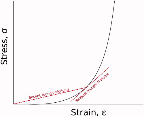
Figure 2. Schematic illustrating the relationship of stiffness and IOP. This graph visually depicts how a more compliant cornea (dashed line) at a higher IOP (triangle on dashed line) may exhibit a stiffer response (greater resistance to deformation) than a cornea with stiffer properties (solid line) at lower IOP (triangle on solid line).Citation9
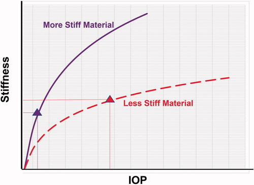
Figure 3. Schematic illustrating mechanical hysteresis. This curve demonstrates the different pathways taken during the loading and unloading phases of a nonlinearly elastic material. Mechanical hysteresis, the energy lost due to internal friction of the material, is the difference between these two pathways and is represented by the shaded area between the loading and unloading curves.
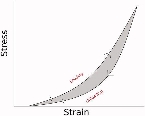
Figure 4. The mean stress-strain behavior of the corneas in Zheng’s study. Note that the treated group (black) exhibited a shift to the right from control (white), indicating a reduced resistance to deformation and greater strain for a given stress, compared to the control groups.Citation36
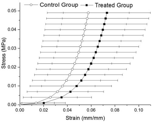
Figure 5. Example of an ORA measurement. As the cornea deforms under an air puff, the infrared (IR) applanation signal (red) represents the light collected by the detector with the corresponding geometry of the cornea shown at the top. Also plotted is the air-pressure signal (blue). As the cornea applanates, the light generates the first peak on the detector. The applanation signal then decreases as the cornea enters a state of slight concavity and peaks again in the outgoing direction during unloading, as the cornea goes through applanation a second time as it recovers its convex shape. P1 and P2 are the corresponding applanation pressures and Pmax is the maximum pressure reached.Citation9 Reprinted with permission by Wolters Kluwer Health, Inc.
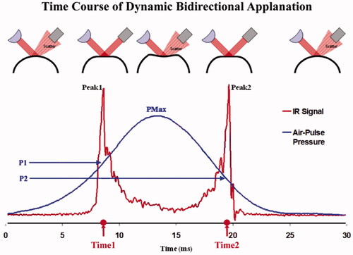
Figure 6. Schematic illustrating corneal hysteresis (CH). Specifically, this term is defined as the difference between inward and outward applanation pressures using the Ocular Response Analyzer (ORA). Pressures at applanation points, A1 and A2, are captured by the ORA during the loading and unloading pathways and used to calculate CH.
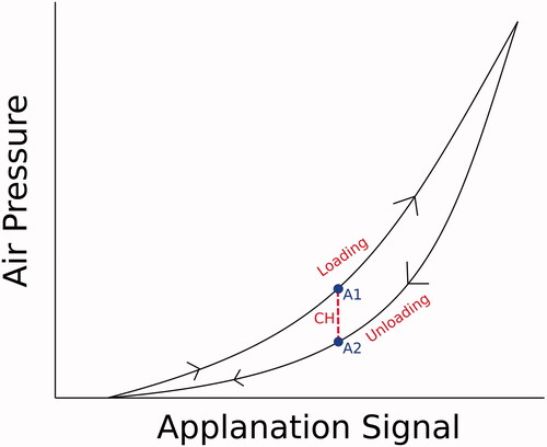
Figure 7. Example of a Corvis ST measurement. As the cornea deforms under an air puff, the high-speed camera captures the changing geometry of the cornea shown at the top. Applanation events are noted as A1 and A2. The oscillation phase begins at the time point when the cornea has reached its limit of maximum deflection and the whole eye begins to move backwards as the air pressure continues to increase.Citation16 Reprinted with permission from SLACK Incorporated.
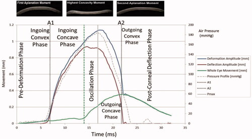
Table 1. Corvis ST parameters are separated into those that are primarily dependent on IOP versus those that are more predominantly influenced by corneal stiffness.Citation16,Citation28,Citation41
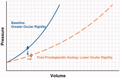
Figure 8. Visual representation demonstrating how a reduction in IOP (vertical arrow) from baseline value (diamond on solid line) to new value (diamond on dashed line) after Prostaglandin Analog (PGA) treatment can be accompanied by an increase in anterior chamber volume (horizontal arrow) if the ocular rigidity drops from a greater value at baseline (solid curve) to a lower value (dashed curve) caused by the reduction in scleral stiffness with PGA treatment.Citation33