Theoretical Response of Laser Aerosol Spectrometers and Data Inversion by Stochastic Reconstruction

Figures & data

FIG. 1 Conversion factors for each calibration particle size, together with the fitting function.

TABLE 1 Conversion factors for the LAS-X and HSLAS

Parameter	LAS-X	HSLAS
A	1.36	5.19
B	0.20	0.37
C	0.56	0.56

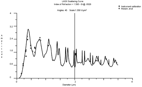
FIG. 2 Calculated scattering amplitude for PSL as a function of particle diameter using manufacturer's calibration data and measurements of Reisert et al. The points at 2.02 μ m do not affect the scale factor.

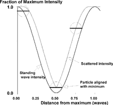
FIG. 3 Illustration of the passage of 0.05 μ m particles between intensity maxima of the standing-wave pattern with the resulting scattered light intensity. The curve for scattered intensity corresponds to particles whose centers pass a distance from the standing wave maxima.

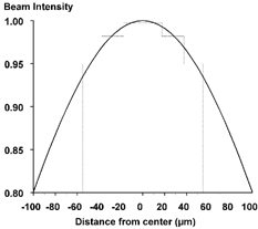
FIG. 4 Intersection of the particle beam with the laser intensity profile. The three equal area bands have average intensities of 0.998, 0.982, and 0.950 of the maximum laser beam intensity.

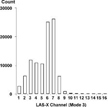
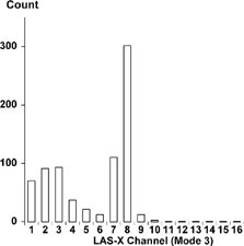
FIG. 5 LAS-X counts using a lab-generated PSL aerosol, nominally 0.70 μ m diameter. The nominal boundaries for Channel 8 are 0.5 and 0.65 μ m. Counts in Channels 1–5 are probably due to surfactant in the PSL solution.

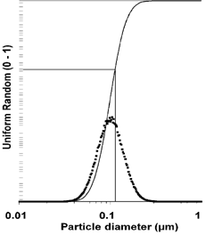
FIG. 6 A uniform deviate between 0 and 1 selects a fraction on the cumulative curve. The diameter bin that corresponds to the fraction is incremented. The resulting histogram resembles the derivative of the cumulative curve, but it has been constructed randomly.

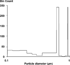
FIG. 7 Starting bin approximation for channel count data. The initial bin counts are determined by dividing the channel count data by the number of bins contributing to each channel. The narrow bin count at 0.93 μ m is produced by a small dip, shown in Figure 2 at the same size, that barely drops into Channel 8.

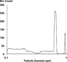
FIG. 8 First stochastic reconstruction of the channel data. The cumulative distribution constructed from Figure 7 was smoothed before these data were generated. This curve is the average of three separate reconstructions using the same cumulative curve. A final smooth was applied to the average.

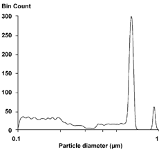
FIG. 9 Fourth stochastic reconstruction of channel data. The cumulative distributions from each prior reconstruction were smoothed. This curve is the average of three separate reconstructions using the latest cumulative curve. A final smooth was applied to the average.

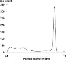
FIG. 10 Twentieth stochastic reconstruction of channel data. The cumulative distributions from each prior reconstruction were smoothed. This curve is the average of three separate reconstructions using the latest cumulative curve. A final smooth was applied to the average. The narrow initial peak at 0.93 μ m has been smoothed away.

TABLE 2 Results of fitting single channel data using 1.593 + 0i

	#						Relative
	Initial	Total	Peak	FWHM	Mean peak	Standard	standard
Channel	peaks	count	(μ m)	(μ m)	count	deviation	deviation
1	1	36800	0.113	0.019	894	1.5	0.002
2	1	30000	0.146	0.020	884	2.2	0.002
3	1	30000	0.185	0.031	773	2.0	0.003
4	1	30000	0.229	0.031	882	2.9	0.003
5	1	30000	0.272	0.034	950	1.6	0.002
6	1	30000	0.326	0.053	751	1.6	0.002
7	1	30000	0.447	0.215	286	2.5	0.009
8	2	30000	0.639	0.057	1249	0.5	0.000
9	3	30000	0.707	0.345	513	1.4	0.003
10	4	30000	1.565	0.108	581	3.7	0.006
11	6	30000	1.140	0.121	679	1.5	0.002
12	3	30000	2.110	0.087	870	3.7	0.004
13	4	30000	2.223	0.463	523	4.1	0.008
14	5	30000	3.235	0.117	682	5.0	0.007
15	10	30000	2.935	0.196	646	3.6	0.006
16	6	30000	3.435	0.154	592	2.8	0.005

FIG. 11 Synthesized channel data from 10,000 “particles” each at 0.48, 1.09, and 2.8 μ m.

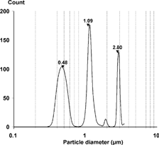
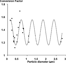
FIG. 12 Reconstruction of synthesized channel data from Figure 11. The triangles indicate the diameters that generated the data in Figure 11.

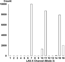
FIG. 13 Counts obtained by dilution for titanium dioxide pigment from a production line.

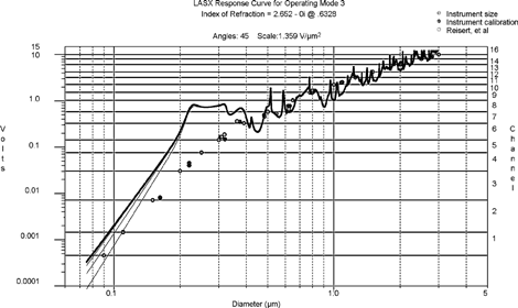
FIG. 14 Calculated LAS-X voltage response to spherical TiO₂ particles with index of refraction 2.652 − 0i. The individual curves for the interference calculations are shown below 0.3 μ m. The horizontal lines define the channel voltage thresholds.

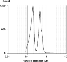
FIG. 15 Reconstructed TiO₂ size distribution, using a 2% smoothing parameter.