A Design Tool for Aerodynamic Lens Systems

Figures & data

FIG. 1 Schematic and nomenclatures of the lens system.

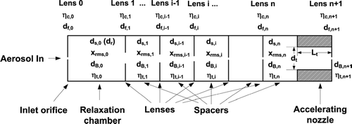
FIG. 2 Near-axis particle contraction factor as a function of the Stokes number for various Reynolds numbers at three different subsonic Mach numbers. (a) Ma = 0.03; (b) Ma = 0.10; (c) Ma = 0.32.

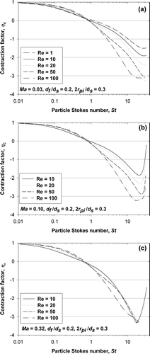
FIG. 3 Optimum Stokes number as a function of Reynolds number for three different Mach numbers.

FIG. 4 The operating pressures for focusing unit density particles of different sizes as a function of orifice size using (a) air and (b) helium as the carrier gas. The flowrate is 0.1 slm. The two dash lines are the lower pressure limits p _Ma and p _Kn, respectively. The solid lines are p _focusing for indicated sizes.

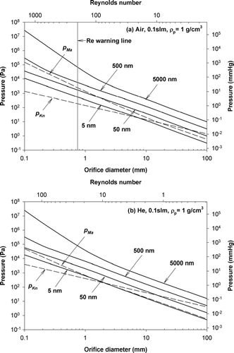
FIG. 5 Streamlines through two lenses separated by a spacer.

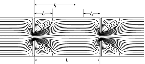
FIG. 6 Reattachment length of flow downstream of an axisymmetric expansion.

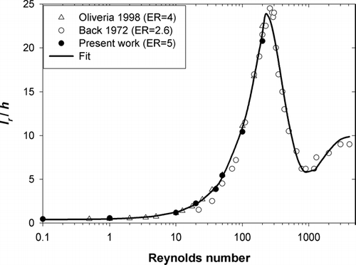
FIG. 7 Straight bored critical orifice and cylindrical relaxation chamber. (a) Flow streamlines and illustration of the half jet opening angle; (b) Trajectories of 100 nm (above axis) and 1 μ m (below axis) particles.

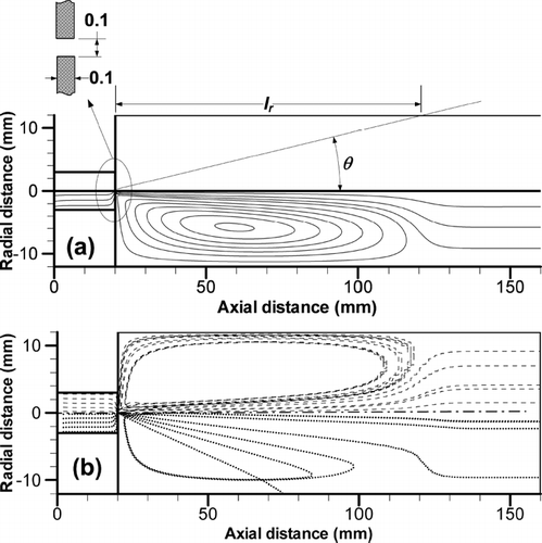
FIG. 8 Modified relaxation chamber with a conical divergent section to reduce recirculation and particle loss. (a) Flow streamlines (straight orifice); (b) Trajectories of 100 nm (above axis) and 1 μ m (below axis) particles (straight orifice); (c) Trajectories of 100 nm (above axis) and 1 μ m (below axis) particles (orifice with a chamfer).

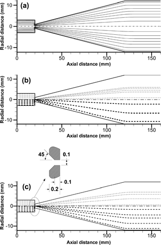
FIG. 9 Normalized particle terminal axial velocities downstream of several aerodynamic lens systems.

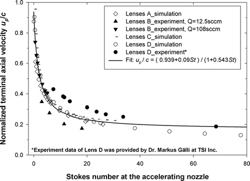
TABLE 1 Key features of four lens assemblies with step accelerating nozzles used in particle axial velocity comparison

Lens system	d n (mm)	d s (mm)	d t (mm)	L t (mm)	Gas	p 1 (Pa)	d p (nm)
A (Wang et al. 2005b)	2.76	10	6	5	He	528	3–30
B (Liu et al. 1995b)	3.0	10	6	10	Air	93–333	25–250
C (TSI AFL-050)	3.2	17.78	7.62	17.78	Air	250	50–500
D (TSI AFL-100)	1.48	17.78	7.62	17.78	Air	600	100–3000

FIG. 10 Particle transmission efficiency as a function of the Stokes number for various Reynolds numbers at three different subsonic Mach numbers. (a) Ma = 0.03; (b) Ma = 0.10; (c) Ma = 0.32.

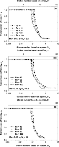
FIG. 11 Cutoff Stokes numbers as a function of Reynolds number for three different Mach numbers.

FIG. 12 Flow chart for the aerodynamic lens design module.

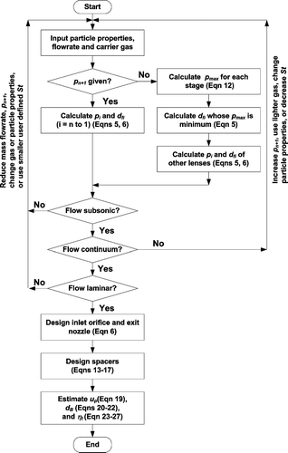
TABLE 2 Key features of the three aerodynamic lens systems used for the lens design tool validation

Lens system	d f (mm)	p 1 (Pa)	d p (nm)	Q STP (slm)
1 (Wang et al. 2005)	1.26, 1.64, 2.33, 2.76	528	3–30	0.1
2 (Liu et al. 1995)	5.0, 4.5, 4.0, 3.75, 3.5, 3	291	25–250	0.108
3 (Schreiner et al. 2002)	1.4, 1.2, 1.0, 0.8, 0.7, 0.6, 0.5, 0.4	5000	300–5000	0.052

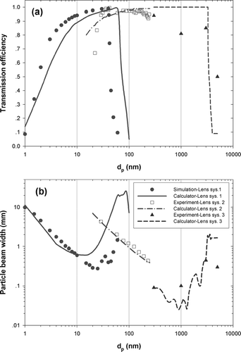
FIG. 13 Comparison of the lens calculator prediction with experimental or numerical evaluation for three lens systems in the literature. (a) Transmission efficiency; (b) Particle beam width. The legends of the two figures are the same.

Wang , X. , Gidwani , A. , Girshick , S. L. and McMurry , P. H. 2005b . Aerodynamic Focusing of Nanoparticles: II. Numerical Simulation of Particle Motion through Aerodynamic Lenses . Aerosol Sci. Technol. , 39 ( 7 ) : 624 – 636 . [CROSSREF] [CSA]

 Web of Science ®Google Scholar

Liu , P. , Ziemann , P. J. , Kittelson , D. B. and McMurry , P. H. 1995b . Generating Particle Beams of Controlled Dimensions and Divergence: II. Experimental Evaluation of Particle Motion in Aerodynamic Lenses and Nozzle Expansions . Aerosol Sci. Technol. , 22 ( 3 ) : 314 – 324 . [CSA]

 Web of Science ®Google Scholar

Wang , X. , Kruis , F. E. and McMurry , P. H. 2005a . Aerodynamic Focusing of Nanoparticles: I. Guidelines for Designing Aerodynamic Lenses for Nanoparticles . Aerosol Sci. Technol. , 39 ( 7 ) : 611 – 623 . [CROSSREF] [CSA]

 Web of Science ®Google Scholar

Schreiner , J. , Voigt , C. , Zink , P. , Kohlmann , A. , Knopf , D. , Weisser , C. , Budz , P. and Mauersberger , K. 2002 . A Mass Spectrometer System for Analysis of Polar Stratospheric Aerosols . Rev. Scientif. Instruments , 73 ( 2 ) : 446 – 452 . [CROSSREF] [CSA]

 Web of Science ®Google Scholar