Graphical Analysis of the Performance of Venturi Scrubbers for Particle Abatement. Part II: Size Distribution of Penetrating Particles

Figures & data

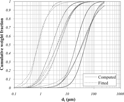
FIG. 1 Normalized cumulative weight distributions of penetrating particles predicted by the Calvert theoretical model and optimally fitted by lognormal distributions.

FIG. 2 (a) Nomographs based on the Calvert formulation, for Bf = 1.4, yielding the output particle distribution parameters G _c d _pα and lnσ _p as function of the input particle distribution parameters G _c d _mα and lnσ _g . (b) Nomographs based on the Calvert formulation, for Bf = 1.6, yielding the output particle distribution parameters G _c d _pα and lnσ _p as function of the input particle distribution parameters G _c d _mα and lnσ _g . (c) Nomographs based on the Calvert formulation, for Bf = 1.9, yielding the output particle distribution parameters G _c d _pα and lnσ _p as function of the input particle distribution parameters G _c d _mα and lnσ _g . (d) Nomographs based on the Calvert formulation, for Bf = 2.3, yielding the output particle distribution parameters G _c d _pα and lnσ _p as function of the input particle distribution parameters G _c d _mα and lnσ _g . (e) Nomographs based on the Calvert formulation, for Bf = 3, yielding the output particle distribution parameters G _c d _pα and lnσ _p as function of the input particle distribution parameters G _c d _mα and lnσ _g . (f) Nomographs based on the Calvert formulation, for Bf = 4, yielding the output particle distribution parameters G _c d _pα and lnσ _p as function of the input particle distribution parameters G _c d _mα and lnσ _g . (g) Nomographs based on the Calvert formulation, for Bf = 6, yielding the output particle distribution parameters G _c d _pα and lnσ _p as function of the input particle distribution parameters G _c d _mα and lnσ _g . (h) Nomographs based on the Calvert formulation, for Bf = 16, yielding the output particle distribution parameters G _c d _pα and lnσ _p as function of the input particle distribution parameters G _c d _mα and lnσ _g .

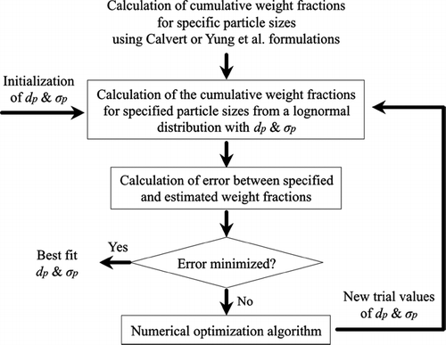
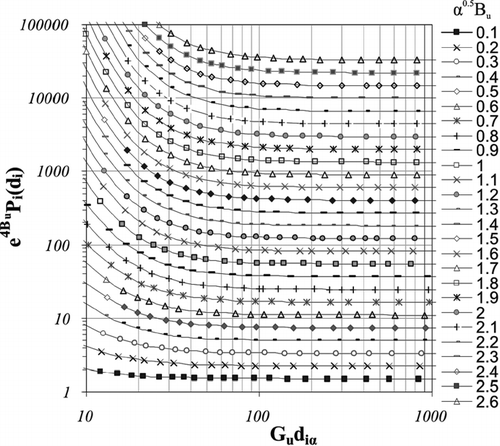
FIG. 3 Algorithm for generating best-fit lognormal distribution parameters d _p and σ _p from cumulative weight fraction series computed through the use of Calvert and Yung et al. formulations.

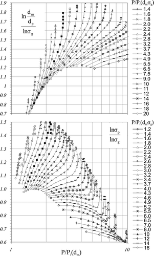
FIG. 4 Nomograph yielding the fractional penetration parameter e ^{4B _u} P _i (d _i ), based on the Yung et al. efficiency formulation, as function of the parameters G _u d _iα and α^0.5 B _u.

FIG. 5 Nomographs based on the Yung et al. efficiency formulation, yielding the output particle distribution parameters lnd _m /d _p /d _p /ln σ _g and ln σ _p /ln σ _g , as function of parameters P/P _i (d _m ) and P/P _i (d _m σ _g ).