A Thermophoretic Precipitator for the Representative Collection of Atmospheric Ultrafine Particles for Microscopic Analysis

Figures & data

FIG. 1 Exploded schematic cross section of the precipitator; (a) Along the center of the precipitator, following the flow. b: Across the center of the precipitator, perpendicular to the flow. (c) Top view of the Peltier Assembly with cover sheet, Aluminum spacer, and sealing.

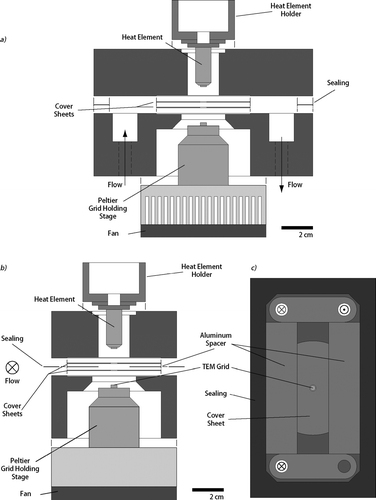
FIG. 2 Details of the precipitator's design. (a) Enlargement of the sample channel. (b) Schematic representation of the precipitator's periphery.

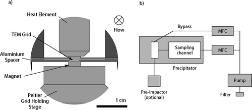
FIG. 3 Key elements of the numerical model. (a) Parabolic flow profile inside the sampling channel. At flow speeds of 2 l/min and a temperature gradient of 4· 10⁵ K m^{− 1} only particles from the grey area are sampled. (b) Principle parameters of the model. Starting coordinates of the particles are randomly generated in the “starting area.”

FIG. 4 Deposition pattern as calculated by the model based on particle trajectories. Colors indicate the local deposition efficiency of a respective matrix cell relative to the average of the grid. The curved shape of areas with similar deposition efficiency is due to the circular geometry of the cold and hot plate. The deposition gradient is a consequence of the parabolic velocity profile.

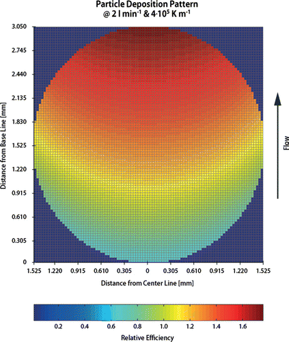
FIG. 5 Schematic representation of the facility for generating Ag aerosols. (a) Setup for polydisperse aerosols. SMPS: scanning mobility particle sizer; MFC: mass flow controller. (b) Setup for monodisperse aerosols. DMA: dynamic mobility analyzer; CPC: condensation particle counter.

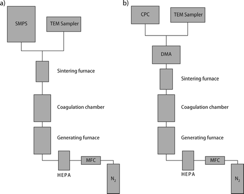
FIG. 6 Quantitative comparison of particle size distributions measured by the SMPS and calculated from TEM/image analysis using the described model. The black lines represent the SMPS scans, the grey lines the TEM analysis and the black circles represent the Gaussian fit of the TEM/image analysis data. The particle number concentration of the aerosol determined by TEM image analysis in combination with the model lies within 10% of the SMPS results.

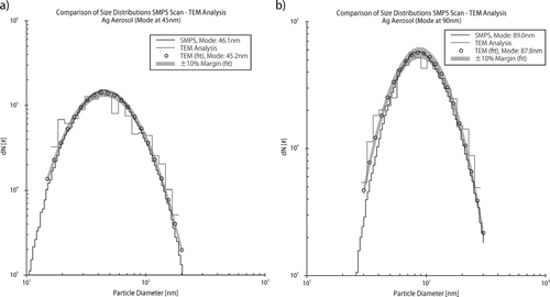
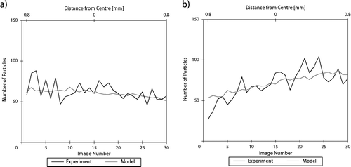
FIG. 7 Comparison of the calculated and measured particle deposition pattern using polydisperse Ag aerosols. The sample for Figure (a) was taken with a temperature gradient of 4· 10⁵ K m⁻¹ and the sample for Figure (b) with a temperature gradient of 3.3· 10⁵ K m⁻¹.

FIG. 8 Quantitative comparison of calculated and measured particle numbers from monodisperse Ag aerosols (particle diameters a: 80 nm; b: 40 nm). The micrographs for particle counting were taken along a transect.