Figures & data
FIG. 1 Relative photoacoustic signals compared to no evaporation at surface pressure, 295 K, and a photoacoustic frequency of 1 kHz. The upper panel shows various values of the mass accommodation coefficient and the lower curve shows various relative humidities. The heavy curve is repeated between the panels. The case for 274 K and 75% RH has the same absolute humidity as 295 K and 20% RH.
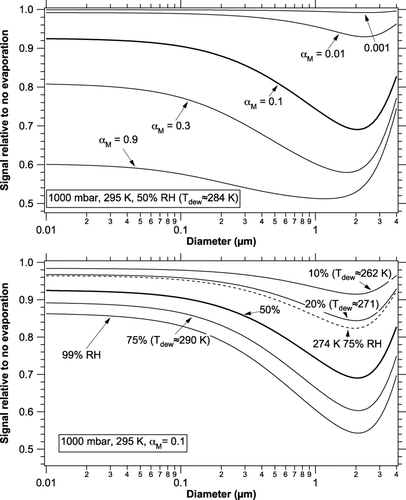
FIG. 2 The effect of internal heat capacity on the photoacoustic signal at 1 kHz for particles with the specific heat of water. Internal heat capacity is more important for a small mass accommodation coefficient because then latent heat transfer does not help heat and cool a particle.
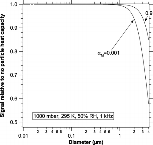
FIG. 3 Temperature rise and mass loss of water (dotted curve) from highly absorbing particles during a single photoacoustic cycle for conditions typical of the NOAA photoacoustic instrument. The dashed curve shows the amount of heating for a lower pressure case, as might occur during an aircraft measurement or downstream of a critical orifice.
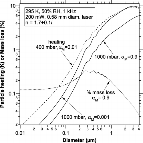
FIG. 4 Dew point dependence of the change in photoacoustic signal due to evaporation. Calculations were done at 50% RH, 1 kHz, and a range of temperatures (8 to 12 K greater than the dew points). Curves are shown for 50 and 500 nm diameter particles.
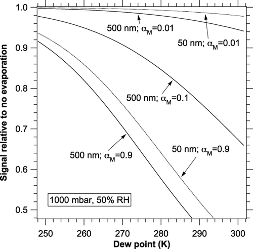
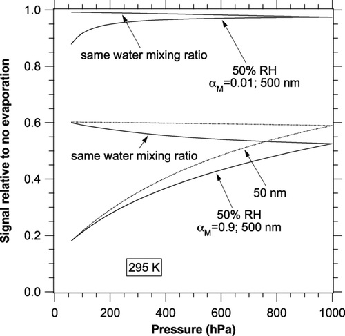
FIG. 5 Pressure dependence of the change in photoacoustic signal due to evaporation. Calculations were done at 295 K and 1 kHz. Curves are shown for both constant RH and constant water mixing ratio. For α M = 0.01 the values for 50 nm diameter particles (not shown) are larger than those for 500 nm particles.