Figures & data
FIG. 1 Snapshots of the system during the ballistic coalescence phase. The volume fraction if f v = 0.001. 2D projections of part of the system are shown at Monte Carlo time steps 0, 5000, 40,000, respectively. The apparent overlap is due to projection of the 3d volume onto a 2d surface; all clusters are spherical.
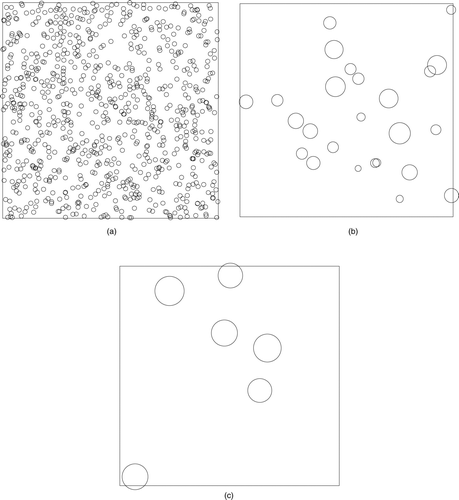
FIG. 2 Number of particles N c (t D ) versus time t D shown in a log-log plot during coalescence with a ballistic movement of the particles. The slope of the straight line yields the kinetic exponent z = 1.2.
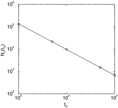
FIG. 3 Number of particles N c (t D ) versus time t D shown in a log-log plot during coalescence with a diffusive movement of the particles. The slope of the straight line yields the kinetic exponent z = 1.
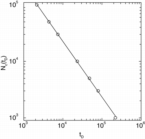
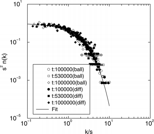
FIG. 4 Scaled form of ballistic and diffusive particle size distributions at t D for various values of t D . The scaled distribution has the functional form ϕ (x) = Ax− λe- α x for large sizes (x > 1) with α = 1 – λ with ≈ (ballistic coalescence) = 1/6 and λ (diffusive coalescence) = 0.
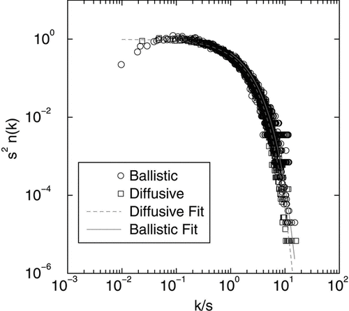
FIG. 5 A typical cluster formed from DLCA with ballistic monomer mass distribution. This snapshot was taken at 2,000,000 time steps.
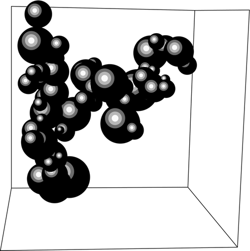
FIG. 6 Log-log plot of inverse cluster count N c − 1(t) − N c − 1(t = 0) versus time t for mono-disperse DLCA and DLCA with poly-disperse distributions originating from both ballistic and diffusive coalescence as discussed before. Slope for each of these curves yields z = 1 in agreement with diffusive scaling. Since the number of monomers at this DLCA stage is much smaller than in the coalescence phase, we compute inverse cluster count N c − 1(t) − N c − 1(t = 0) instead of just the cluster number N c (t). At final times (t D = 100,000 for diffusive coalescence and t D = 40,000 for ballistic coalescence) both diffusive and ballistic coalescence yield an average particle diameter of 7σ.
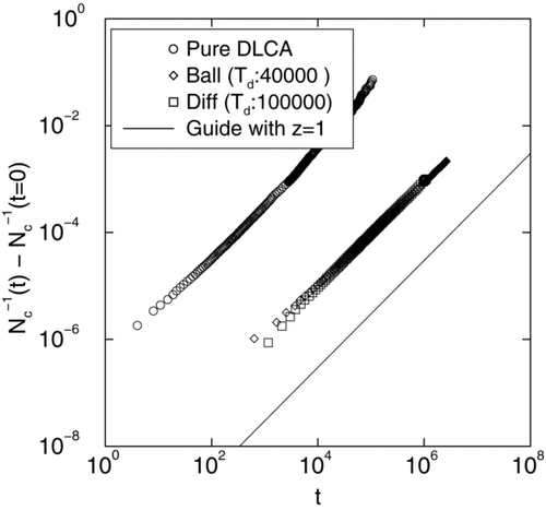
FIG. 8 (a) Log-log graph of mass of the clusters M rescaled by the average particle mass < m > versus the radius of gyration of the clusters rescaled by the average particle radius < r > for ballistic coalescence initial particle distributions. There are two distinct zones in this graph. Below Rg/〈 r 〉 = 1 the clusters are compact (dimers, trimers, and other small non-fractal clusters) and yield an exponent of D f = 3. Above this value of Rg/〈 r〉, the straight line fit to the data yields D f = 1.7± 0.1. (b) Same as in 8 (a) except for diffusive coalescence initial particle distributions. As before, there are two distinct zones in this graph. Below Rg/〈 r〉 = 1 the clusters are compact (dimers, trimers, and other small non-fractal clusters) and yield an exponent of D f = 3. Beyond this value of Rg/〈 r〉, the straight line fit to the data yields D f = 1.7± 0.1.
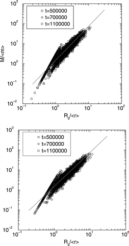
FIG. 7 Log-log plots of average radius of gyration of clusters < R g > versus time t for mono-disperse DLCA and DLCA with poly-disperse distributions originating from both ballistic and diffusive coalescence. The straight line part for all three curves yield an exponent of υ = 0.55.
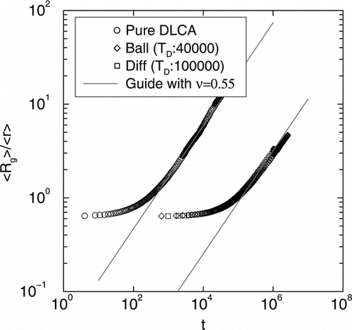
FIG. 9 Scaling of DLCA with ballistic and diffusive monomer mass distributions. Scaling function is ϕ (x) = x − λ e − α x with λ = 0 agrees well with the data.