Determination of the Mean Mobility of Aerosol Nanoparticles Classified by Differential Mobility Analyzers

Figures & data

FIG. 1. Illustration of DMA sizing error. When a voltage V₁ is applied to the DMA, particles from the tail of the aerosol population with mobilities in the common region under the original distribution f₀(Z) and the transfer function Ω(V₁, Z) are classified/detected. A mobility Z₁(V₁), given by Equation (1)[1] , is assigned to these particles in spite that there are no particles with such a high mobility in the aerosol population.

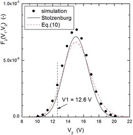
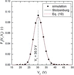
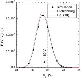
FIG. 2. Example of particle classification with a single DMA. f₀ is the mobility distribution of the aerosol. Ω_nd is the ideal transfer function for non-diffusive particles; Ω is the transfer function calculated by: Stolzenburg's model (solid line), MonteCarlo simulation (dots), and lognormal approximation (8) (dashed line); f₁ is the fraction of particles of mobility Z classified at voltage V₁ divided by dlnZ, calculated from Equation (4)[4] using the transfer function calculated by: Stolzenburg's model (solid line), MonteCarlo simulation (dots), and lognormal approximation (8) (dashed line). The theoretical mobility directly inferred from the applied voltage and Equation (1)[1] is denoted as Z₁; the true mobility of the classified particles is shown as Z_{1, true}. Data obtained for the Nano-DMA of Chen et al. (1998) operated at Q_a/Q_sh = 2/20 (in lpm) and V₁ = 12.6 V; aerosol mobility distribution: Z_g0 = 0.25cm²/Vs (D_pg = 2.9 nm); σ_g0 = 1.2.

FIG. 3. Example of particle classification by DMA-2 keeping fixed the voltage V₁ (12.6 V) applied to DMA-1. In this case, the particles withdrawn from DMA-1 were extracted from the high-mobility tail of the distribution. Data obtained for the Nano-DMA operated at flow rate ratio of 2/20; aerosol mobility distribution: Z_g0 = 0.25 cm²/Vs and σ_g0 = 1.2.

FIG. 4. Same as Figure 3, except that the particles withdrawn from DMA-1 were extracted from a region close to the peak of the distribution (V₁ = 30.3 V).

FIG. 5. Same as Figure 3, except that the particles withdrawn from DMA-1 were extracted from the low-mobility tail of the distribution (V₁ = 60.0 V).

FIG. 6. Comparison between the true mobility of particles classified by DMA-1 calculated from MonteCarlo simulations by two approaches, using (i) Equation (5)[5] (y-axis), and (ii) Equations (2)[2] and (7)[7] (x-axis). Data obtained for the Nano-DMA (triangles: Q_a/Q_sh = 1/10; squares: 2/20) with Z_g0 = 0.25 cm²/Vs and σ_g0 between 1.1 and 1.8; and the Vienna type DMA (circles) operated at Q_a/Q_sh = 2/20, with Z_g0 = 0.20 cm²/Vs and σ_g0 between 1.2 and 2.0.

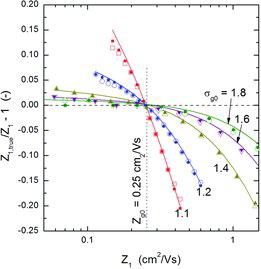
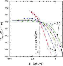
FIG. 7. Comparison between the mobility calculated with Equation (1)[1] and the true mobility of particles classified with a DMA. Nano-DMA operated at a flow rate ratio of 1/10. The MonteCarlo simulation results are represented by open symbols; those obtained using the rigorous (i.e., not the lognormal approximation) transfer function of Stolzenburg are plotted with solid symbols. The solid curves were calculated using Equation (9)[9] . The aerosol had a mean geometric mobility of 0.25 cm²/Vs (mobility-equivalent particle diameter of 2.9 nm) and the geometric standard deviations shown in the plot.

FIG. 8. Same as Figure 7, but in this case the Nano-DMA was operated at an aerosol-to-sheath flow rate ratio of 2/20.

FIG. 9. Same as Figures 7 and 8, but using the Vienna type DMA operated at an aerosol-to-sheath flow rate ratio of 2/20. The aerosol had a mean geometric mobility of 0.20 cm²/Vs (mobility-equivalent particle diameter of 3.3 nm) and the geometric standard deviations shown in the plot.

Chen, D.R., Pui, D.Y. H., Hummes, H., Fissan, H., Quant, F.R., and Sem, G.J. (1998). Design and Evaluation of a Nanometer Aerosol Differential Mobility Analyzer (Nano-DMA). J. Aerosol Sci., 29:497–509.

 Web of Science ®Google Scholar