Aerosol Filtration with Mobility-Classified Particles: Role of Multiply Charged Particles in Skewing Penetration Measurements

Figures & data

TABLE 1 Test particle and filter characteristics used in the modeling study

Particle size distribution, dN/dlogDp			Filter penetration, P
Label	Dpg	σpg	Label	Dfg	σfg
SD1	150	1.6	FP1	50	1.6
SD2	150	1.1	FP2	300	1.2
SD3	10	1.6	FP3	300	1.6
			FP4	50	1.2

FIG. 1. Filter penetrations calculated using Equation (12) compared against actual penetration distributions. The filter penetration characteristics for the two test cases shown are (a) FP1 and (b) FP2 as described in Table 1. For both cases, the test particles have a size distribution SD1 and the DMA is operated with sheath and aerosol flowrates of 3.0 and 0.3 l min⁻¹, respectively. In the legend, P_A is the actual filter penetration and P₀ is filter penetration calculated based on Equation (12).

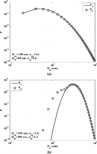
FIG. 2. (a) The fraction of singly charged particles upstream and downstream of the test filter. The test particle size distribution is SD1 and the filter penetration distribution is FP3. (b) The multiple-charge penetration factor F for a filter with penetration distribution of FP3 and test particles with size distribution of SD1, SD2, and SD3. (c) The multiple-charge penetration factor F for particles with size distribution SD1 and filters with penetration distributions of FP1, FP2, FP3, and FP4.

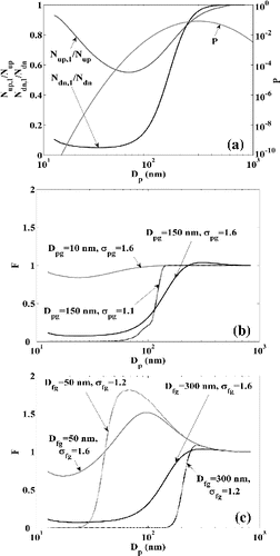
FIG. 3. Relative error under different upstream particle size distributions with the assumption of singly charged particles and filter penetration characteristics of (a) FP4, (b) FP1, (c) FP2, and (d) FP3.

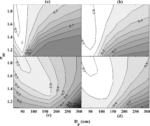
FIG. 4. Filter penetrations calculated using Equation (12) with different DMA resolutions. Here the results obtained from DMA resolution (Q_sh/Q_a) of 3 and 10 are labeled as R = 3 and R = 10, respectively. The test particle and filter characteristics are SD1 and FP2.

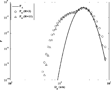
FIG. 5. The penetrations calculated with multiple-charge correction algorithm compared against the actual penetration and the penetration obtained with singly charged particle assumption. The particles have distribution of SD1 and the filter penetration characteristics are described by (a) FP1, and (b) FP2. Here P₁ is the corrected filter penetration, obtained from Equation (19), considering the multiple-charge contribution.

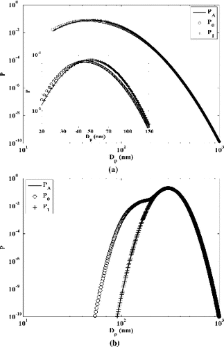
FIG. 6. Filter penetrations calculated for the cases of coarse DMA channels and for the case of limited DMA classification range (maximum classification size of 400 nm singly charged equivalent diameter). The test particles characteristics are assumed to be SD1 and the filter penetrations (a) FP1, and (b) FP2.

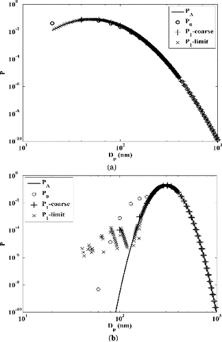
FIG. 7. Schematic diagram of the experimental setup for filter penetration measurements.

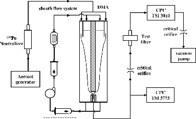
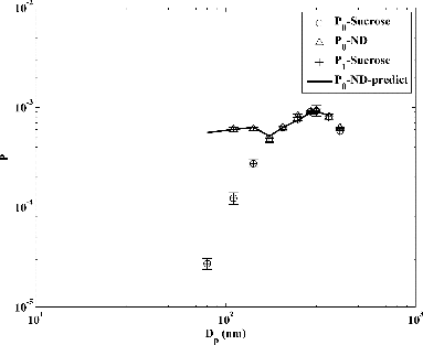
FIG. 8. Filter penetration measurements made at a pressure of 7.6 kPa and a flowrate of 1.0 l min⁻¹ with sucrose and polystyrene latex (PSL) particles generated using an electrospray. The penetrations calculated using Equation (12) with Sucrose and 200 nm PSL particles are labeled P₀-Sucrose and P₀-ND, while the multiple-charge corrected penetrations for the sucrose particles is labeled as P₁-Sucrose. Using the P₁-Sucrose penetration curve, the penetration for PSL particles (P₁-ND-predict) is predicted using Equations (9), (10), and (12). The error bars represent the standard deviation of three repeated measurements.