Figures & data
Figure 1. Image analysis process: (a) original image and its histogram; (b) image and histogram after ACC application; (c) image and histogram after adaptive radial convolution, T denotes threshold; (d) segmented image; (e) image with identified fibers.
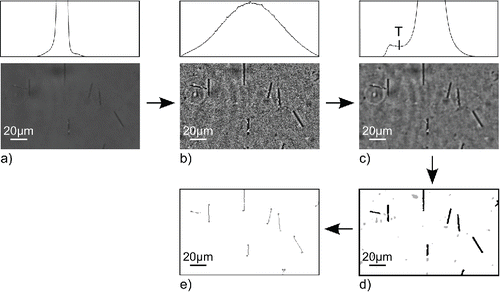
Figure 2. The use of elliptical field to correctly determine the actual size of all counted fibers; dimensions of semimajor and semiminor axis are 0.266 and 0.2 mm (area of about 0.167 mm2).
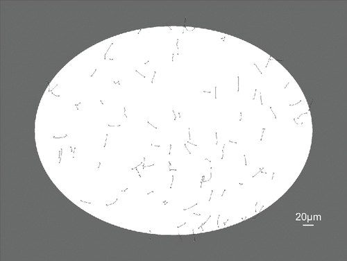
Figure 3. The software interface with six primary windows, the first five windows represent different steps of the IAM, the last window in the bottom right corner displays the results of the analysis.
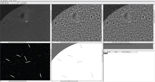
Table 1. Fiber area densities given by analysts for ten samples; SD denotes standard deviation and COV is coefficient of variation.
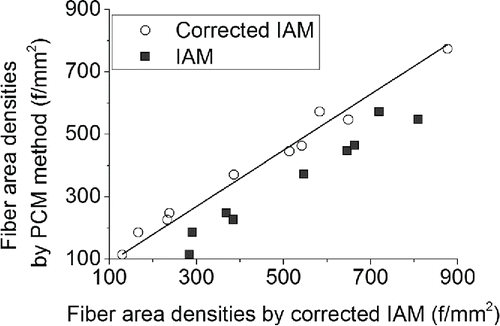
Figure 4. Correlation between the PCM method and the IAM.
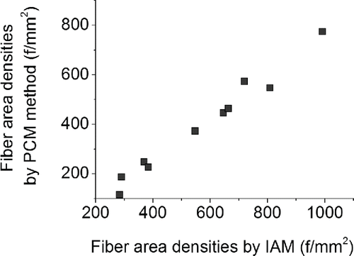
Figure 5. Enhancement of bubble contrast during ACC application; particle image size is 32 × 32 μm.
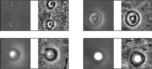
Figure 6. Examples of false identification in three steps of IAM: Original image, application of ACC, fiber identification; (a) crossed fibers, (b) dust particle, (c) crossed fibers, (d) single fiber; particle image size is 24 × 40 μm.
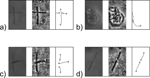
Figure 7. Correlation between the PCM and the corrected IAM.