1,115
Views
10
CrossRef citations to date
0
Altmetric
Original Articles

Mass accommodation coefficients of fresh and aged biomass-burning emissions

, , , , , , ORCID Icon, & ORCID Icon show all
Pages 300-309 | Received 28 Mar 2017, Accepted 06 Nov 2017, Published online: 08 Jan 2018

Figures & data

Table 1. Experimental matrix highlighting the relevant experiments from the FLAME-IV campaign used in this study.

Figure 1. Experimental setup for gas-particle partitioning experiments during the FLAME-IV campaign.
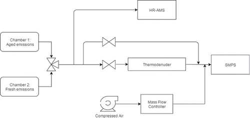
Figure 1. Experimental setup for gas-particle partitioning experiments during the FLAME-IV campaign.

Figure 2. Equilibration profiles for (a) all emissions data, (b) fresh emissions data, and (c) aged emissions data from all experiments after applying the optimization routine. The accommodation coefficients (α) obtained for each case are shown on the respective graphs. Upon binning the scattered data, we see that it follows the behavior of the general dynamic response (GDR) curve.
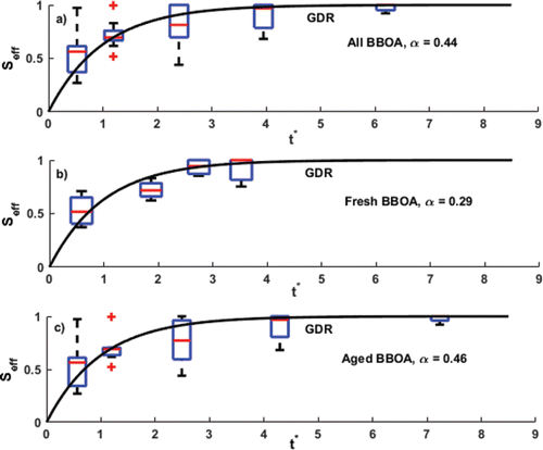
Figure 2. Equilibration profiles for (a) all emissions data, (b) fresh emissions data, and (c) aged emissions data from all experiments after applying the optimization routine. The accommodation coefficients (α) obtained for each case are shown on the respective graphs. Upon binning the scattered data, we see that it follows the behavior of the general dynamic response (GDR) curve.

Figure 3. The binned data from the entire experimental matrix plotted with t* calculated from different values of α. This figure shows the significant deviation from the universal dynamic response with equilibration time scales calculated from logarithmically spaced accommodation coefficient values.
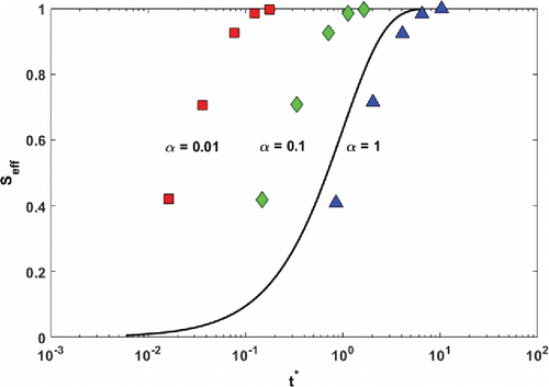
Figure 3. The binned data from the entire experimental matrix plotted with t* calculated from different values of α. This figure shows the significant deviation from the universal dynamic response with equilibration time scales calculated from logarithmically spaced accommodation coefficient values.

Table 2. Mass accommodation values found in this study for biomass burning emissions for different assumptions on molar mass and gas phase diffusion coefficient.

Figure 4. Fractional difference between dynamic and equilibrium cases simulating dispersion of a biomass-burning plume for a range of values of the mass accommodation coefficient α. After about an hour the dynamic and equilibrium cases converge and the relative difference is small regardless of the assumed value of α, but for the best-estimate value (α = 0.44) at no time does the error in the equilibrium partitioning calculation exceed 7%.
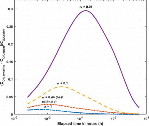
Figure 4. Fractional difference between dynamic and equilibrium cases simulating dispersion of a biomass-burning plume for a range of values of the mass accommodation coefficient α. After about an hour the dynamic and equilibrium cases converge and the relative difference is small regardless of the assumed value of α, but for the best-estimate value (α = 0.44) at no time does the error in the equilibrium partitioning calculation exceed 7%.

Reprints and Corporate Permissions

Please note: Selecting permissions does not provide access to the full text of the article, please see our help page How do I view content?

To request a reprint or corporate permissions for this article, please click on the relevant link below:

Academic Permissions

Please note: Selecting permissions does not provide access to the full text of the article, please see our help page How do I view content?

Obtain permissions instantly via Rightslink by clicking on the button below:

If you are unable to obtain permissions via Rightslink, please complete and submit this Permissions form. For more information, please visit our Permissions help page.