Determination of the aerosol particle size distribution by means of the diffusion battery: Analytical inversion

Figures & data

Figure 1. Original model two-mode spectrum (Equation (35)[35] , modal diameters D₁ = 50 nm, D₂ = 300 nm, and σ₁ = σ₂ = 1.4) (a), and spectra recovered analytically as the sum of lognormal functions Equations (14)[14] and (15)[15] with D_i calculated numerically using Equations (30)[30] , (33)[33] , and (34)[34] (solution 1) (b), and Equations (30)[30] , (34)[34] , (38)[38] , and (40)[40] (solution 2) (c). The contributions from different fractions to the inversely calculated spectra are shown by vertical lines.

Figure 2. Mean single-fiber collection efficiencies for the spectrum Equation (35)[35] (see Figure 1a) as determined directly using the numerically calculated penetrations and formulas Equations (17)[17] and (18)[18] (spheres), using Equation (32)[32] (squares) and Equation (37)[37] (diamonds). Dash lines are spline interpolations of solid symbols.

Figure 3. Original model two-mode spectrum (Equation (35)[35] , Modal diameters D₁ = 50 nm, D₂ = 300 nm, and σ₁ = σ₂ = 1.4) (a), and corrected analytical solutions 1 (b) and 2 (c). Dash lines are lognormal approximations for two main peaks of spectra b and c. The contributions from different fractions to the inversely calculated spectra are shown by vertical lines.

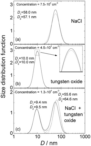
Figure 4. Particle size distributions retrieved from diffusion battery measurements (corrected solutions) for aerosol of NaCl (a), tungsten oxide (b), and mixture NaCl + tungsten oxide (c). Solid line – solution 1, dash line – solution 2, dot lines are lognormal fittings of two-mode spectra components. D₁ and D₂ are geometric mean diameters for single-mode spectra (a and b) and for the components of two-mode spectra (c) for the solutions 1 and 2, respectively.