Figures & data
Table 1. Chamber and particle parameters.
Figure 1. Aerosol number concentration evolution for the six “Standard” experiments (), as compared to a computational model that assumes the 19.0 m3 chamber is spherical (dark gray/red) or cubic (light gray/blue). As model predictions are compared to data, the simulated number concentrations include contributions from coagulation and from wall deposition. The parameter ke, which represents the effect of turbulent mixing in the chamber on the rate of particle wall deposition, was found through the optimization procedure described in the text, where particle charge is neglected (). The optimized results for a spherical and a cubic chamber are essentially identical.
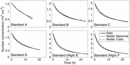
Figure 2. The size-dependent, wall-deposition parameter for a spherical (dashed, dark gray/red) and a cubic (light gray/blue) chamber of the same volume are compared for the six experiments performed under standard operating conditions. These curves were determined by minimizing J with respect to ke (see Section 5.4), thereby fitting observations to simulated predictions. It was assumed that neither an electric field (
) nor any air ions were present. Due to the similarity of these curves, it is sufficient to represent the chamber as a sphere in this work.
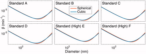
Figure 3. Simulated number-concentration size distributions in the presence of coagulation only (no wall deposition) after 20 h. The initial distribution, shown in solid black/red, matches the initial condition for the “Standard B” experiment and has a total number concentration of ∼2 × 104 cm−3. Simulations were performed both under the assumption that particles have no initial charge (gray line/blue line) and with the assumption that the initial charge distribution satisfies the Wiedensohler formula (circles/black circles). Since the size distributions under these assumptions coincide almost exactly (number concentrations are <0.4% different), one can conclude that the effect of particle charge on the rate of coagulation is negligible for chamber experiments similar to those considered here when there are no ions present.
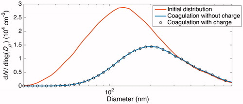
Figure 4. Total number and surface area concentrations after 20 h of coagulation (neglecting wall deposition) at different ion concentrations according to the 7 cases described in are shown in panels (a) and (b), respectively. The initial number concentration and surface area concentration of 2.0 × 104 cm–3 and 2.8 × 103 µm2 cm–3 are displayed as the top dashed line in these panels. These concentrations – excluding the variable concentration of ions present – correspond to the initial condition for the simulations taken from the initial particle distribution of the “Standard B” experiment, which is shown in solid black/red in . The final number and surface area concentrations when no ions are present and each particle has a neutral charge (the Reference Case), shown as the bottom dashed line in the same panels, are 9.2 × 103 cm–3 and 2.4 × 103 µm2 cm–3; the percent difference of the final number and surface area concentrations from these values are shown in panels (c) and (d), respectively. When there is a large difference between the concentrations of the two ion polarities (Case 1–3), the rate of coagulation is dramatically decreased and, therefore, the difference between the coagulated concentrations with and without considering ions and charge is fairly significant. When the difference in concentrations of the two ion polarities are maintained but the absolute concentrations increase, the difference from the Reference Case decreases (Case 4 and Cases 1–3 for the same x). Values for Cases 4 through 7 are shown more clearly in .
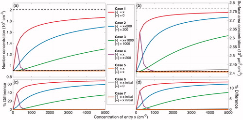
Figure 5. A magnified version of Figure 4 that more clearly displays Cases 4 through 7 (defined in ). Panels (a) and (b) show the total simulated number and surface area concentrations after 20 h of simulated coagulation. The initial distribution corresponds to the beginning of the experiment “Standard B,” but with ions present. In panels (c) and (d), the final number and surface area concentrations for Case 4 through 7 are compared to 9.2 × 103 cm–3 and 2.4 × 103 µm2 cm–3, which are the final total number and surface area concentrations for the Reference Case. When no ion production source is present, as approximated in Cases 6 and 7, there is a negligible effect of the ion concentrations and of charge on coagulation. Even for high ion concentrations, when the two polarities are of equal concentrations (Case 5), there is a small effect of charge. Only when there is a difference between the positive and negative ion concentrations (Cases 1 through and 3), does much of an effect of charge exist. When the difference between the two polarity concentrations remains constant, the effect of charge on coagulation decreases as the absolute concentrations of ions increases (Case 4).
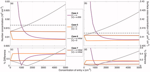
Table 2. Coagulation of the “Standard B” initial particle size distribution with 1.6 nm diameter ions over 20 h.
Figure 6. Simulated particle-number-concentration evolution subject to coagulation and wall deposition for a 20 h experiment. The initial number distribution matches that of the “Standard B” experiment (see ). The effect of assumed electric field strength is shown, based on
s–1. The results indicate that the strength of the electric field is influential, even when relatively small. The black curve shows the number concentration evolution in the absence of an electric field. The gray, dashed curve shows the sole contribution of coagulation to the particle-number-concentration evolution.
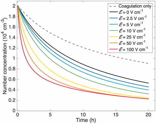
Table 3. Conditions for experiments performed.
Figure 7. Experimental setup for the scanning mobility particle sizer (SMPS) experiments to determine the ratio of positively charged particles of a specific electrical mobility actually in the chamber () to what the steady-state distribution of positively charged particles in the chamber would be (
). Those that pass through the “Chamber” pathway are counted as
, while those that pass through the “Conditioned” pathway are counted as
. The SMPS comprises a differential mobility analyzer (DMA) and a condensation particle counter (CPC).
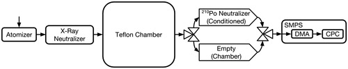
Figure 8. Concentration of positively charged particles that reach the CPC through the “Conditioned” (a) and through the “Chamber” (b) pathway, as shown in . Both and
have units of particle number per cm3 per 0.5 s of the voltage scan. The top axis labels the approximate diameter of transmitted singly and positively charged particles, found using analytical methods (Stolzenburg Citation1988). Since most, but not all, transmitted particles are singly charged, this corresponds only roughly to the size of the particles that reach the CPC. Prior to charge inducement, the chamber was run under standard operating conditions. After 4.1 h of operation, i.e., at 0 h, a static charge was induced on the chamber walls. The first scan after charge inducement is shown in bold. The curves in each panel are separated by 13 min except for those immediately after charge inducement: these are 6.5 min in panel (a) and 19.5 min in panel (b).
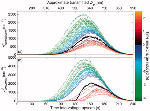
Figure 9. The absence or presence of an electric field within the chamber is discerned by the concentration of positively charged particles that are in the chamber at a given time () as compared to the concentration of positively charged particles from a charge-conditioned version of the same sample (
). Since the same SMPS system was used to measure the concentrations from both pathways, the ratio is calculated as
divided by the average of the two
closest in time. Curves are, therefore, 13 min apart except for the curve immediately after charge inducement (shown in bold), which is 19.5 min apart from the previous one so as to give the most accurate ratio between the before and after inducement cases. As in , the top axis shows the approximate diameter of transmitted singly and positively charged particles, which only inexactly corresponds to the size of the particles that reach the CPC.
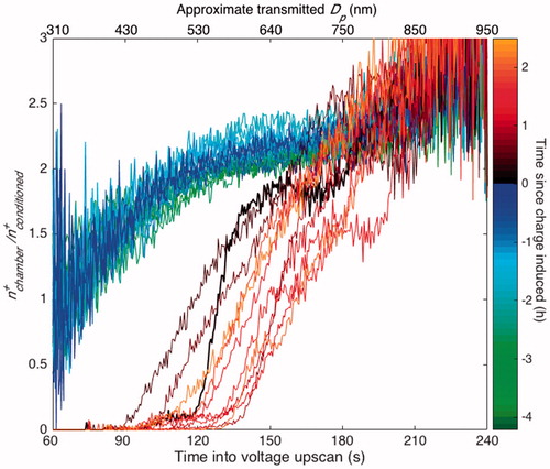
Figure 10. Particle-number-concentration evolution for experiments with approximately the same initial number concentration and size distribution. For humid and standard conditions, the number-concentration evolutions overlap. When a static charge is present, wall deposition occurs much faster and the number concentration decreases more quickly (a). The particle size distribution aligned at a time when all the experiments shown have an approximate number concentration of 1.3 × 104 cm–3 (b) is compared to that distribution about 5 h later (c). All distributions begin similarly, but the particles under static charge conditions deposit much faster. Thus, the evolution in total number concentration, shown in panel (a), is not a result of the difference in the rate of coagulation or in the diameter-dependence of the wall-deposition rate. The difference in the number-concentration evolution, then, is a result only of the electric field strength. Since in a humid experiment, the static charge on the chamber walls is reduced, and therefore decreases any electric field that may be on the chamber, the similarity in wall-deposition rates between the “Humid” and “Standard” experiments indicates that any electric field present in the standard experiments has a negligible effect.
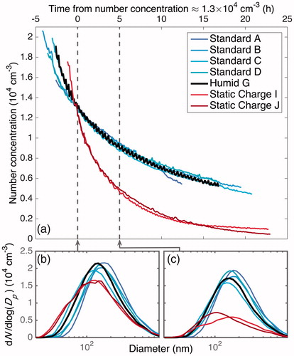
Figure 11. Optimal estimated based on the values of ke and
(given in the legend) when particles are assumed to have an initial charge. Optimized values of
for the experiments performed under standard conditions are close to 0; those for the “Static Charge” experiments are much larger than those for the “Standard” and “Humid” experiments.
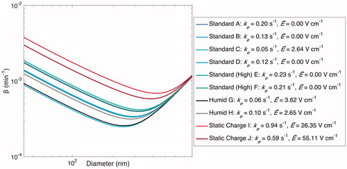
Figure 12. Optimal estimated based on values of ke when particles are assumed to be charge-free. Optimal values of ke are shown in the legend. Note that particles within the chamber may have significant charge, but that this affects the
-curve only when static charge is induced on the chamber walls prior to or during an experiment.
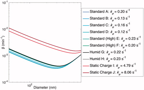
Figure 13. Transformation of to
for the “Static I” experiment using the parameters optimized for that experiment (ke = 0.94 s–1 and
= 26.35 V cm–1).
was determined every 6.5 min. At the beginning of the experiment,
is much larger than that towards the end of the experiment. This difference is particularly pronounced for small particles.
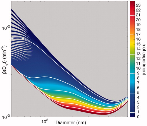
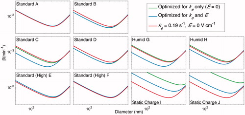
Figure 14. Particle-number-concentration evolution throughout the duration of experiments under standard, humid, and static charge conditions. Data are compared to the simulated number concentration calculated with parameters found from different forms of optimization. Data are given in solid black, and a model with only coagulation included (no wall deposition) is the solid, light, gray curve shown to demonstrate that a significant amount of the loss in number concentration is the result of particle wall deposition. For experiments “A”–“H,” the final selected ke and values of 0.19 s–1 and 0 V cm–1 (light gray, dashed/red), respectively, match well with the number concentrations found by optimizing for only ke while holding
(dark gray, dashed/green) and with that found by optimizing over both ke and
(gray, dashed/blue). In experiments “I” and “J,” the static charge cases, the final selected ke and
values do not match the data well, as expected, because of the strong effect of the electric field on the rate of particle wall deposition. The simulated number concentrations found from optimizing only ke and found from simultaneously optimizing ke and
each match the data well. When
is set to 0, the value of ke compensates until the fit matches the data. This demonstrates the difficulty associated with multiple parameters, especially when each parameter must be determined in the same experiment and may not be extrapolated from one experiment to the next: optimized parameters compensate for one another and lead to much greater uncertainty.
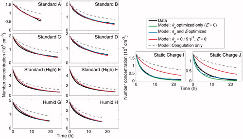
Figure 15. Particle surface area concentration throughout the duration of experiments. The same conclusions as in are drawn here. For all the cases, the optimized models match the data well. Again, for experiments “A”–“H,” the final selected parameters lead to a surface-area-concentration evolution that matches the data but for experiments “I” and “J,” the static charge experiments. Since surface area concentration is used for calculating the rate of vapor uptake in SOA formation experiments, fits of the surface area concentrations using the final selected values of ke and are highly relevant.
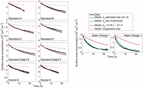
Figure 16. Resulting wall-deposition curves for the final selected parameters (ke = 0.19 s–1 and ) are compared to that determined by minimizing J for each experiment when only ke is allowed to vary (
set to 0) and when both ke and
are subject to optimization. The former represents an uncharged chamber in which the electric field has no effect on the wall deposition. Note that, rigorously speaking, all curves are
, the wall-deposition parameter for neutrally charged particles. Except for the static charge experiments, in which one would expect the charges on particles to be influential, the wall-deposition curve obtained is similar to both the curve found from assuming there is zero charge and from that found assuming charge is present. As in and , the final selected wall-deposition curve fits well for all but the static charge cases.