Figures & data
Figure 1. Illustration of the acoustic agglomerator: (a) homogeneous; (b) nonhomogeneous.
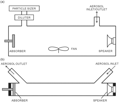
Figure 2. The orthorkinetic (solid), hydrodynamic (dashed), and Brownian (dot-dashed) kernels with respect to the particle size ratio.
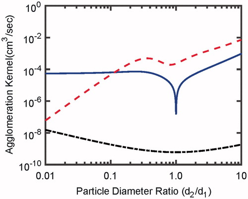
Figure 3. Predictions of the present sectional model (square) compared with the experimental (triangle) and simulation (plus) from Song (Citation1990) for four tests: (a) for HTHP-1, (b) for HTHP-2, (c) for HTHP-3, and (d) for HTHP-4. The initial distribution (diamond) of the aerosol at the chamber inlet is also included.
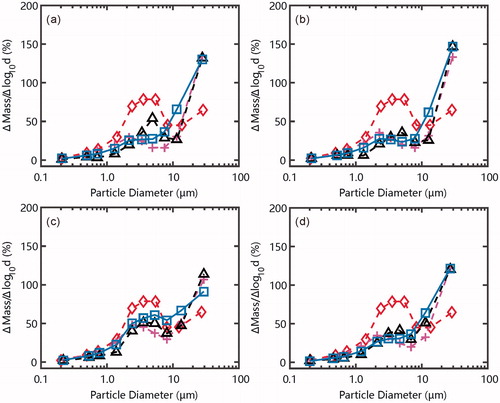
Table 1. Parameters of tests in Song’s acoustic agglomeration experiments.
Figure 4. Illustration of the travelling wave and standing wave in an acoustic agglomerator.
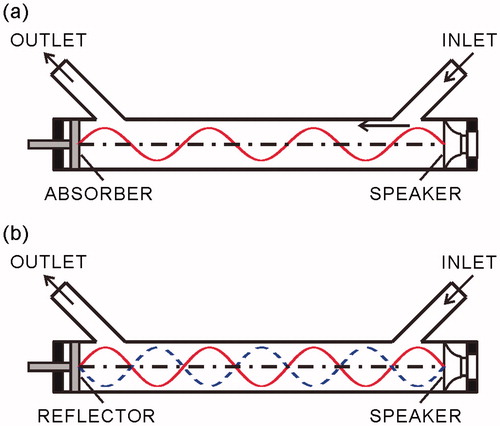
Figure 5. Simulation results (square) compared with experimental measurements (triangle) of the particle size distribution in a standing wave field. The initial distribution (diamond) of the aerosol at the chamber inlet is also included.
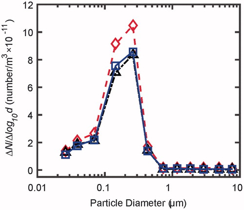
Figure 6. The predicted efficiency of acoustic agglomeration as a function of spatial position along the agglomerator. The agglomeration efficiency is increased in an intermittent way, which is ascribed to the spatial alternation of the acoustic kernel from the velocity node to antinode.
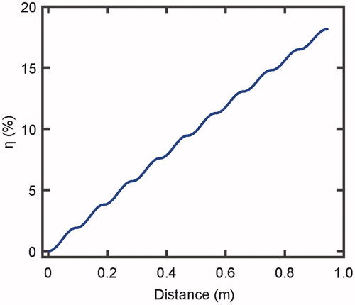
Figure 7. The variation of the attenuation coefficients with respect to the distance from the inlet in the agglomerator at four frequencies: 2 kHz (dotted), 5 kHz (dashed), 10 kHz (dot-dashed), and 21 kHz (solid).
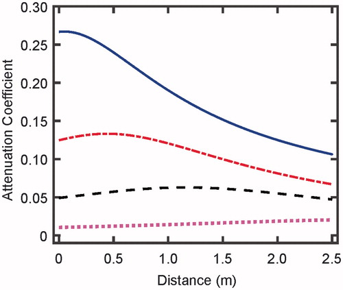
Figure 8. Dependence of the SPL drop on the distance from the inlet in the agglomerator at four frequencies: 2 kHz (dotted), 5 kHz (dashed), 10 kHz (dot-dashed), and 21 kHz (solid).
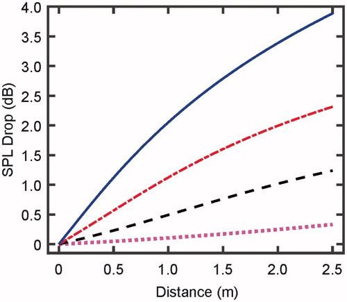
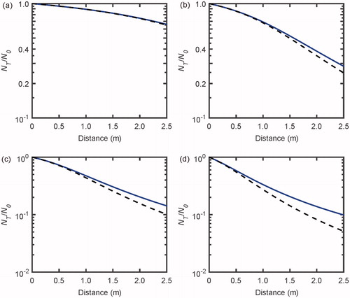
Figure 9. The dependence of the normalized number concentration NT for acoustic agglomeration with (solid line) and without (dashed line) attenuation effect on the space position for four frequencies: (a) 2 kHz, (b) 5 kHz, (c) 10 kHz, and (d) 21 kHz.