Figures & data
Figure 1. FRM samplers located across the continental United States in 2013. The nine sites considered in this study are identified with diamonds. Air Quality System (AQS) site identifications and other sample information is located in online SI (e.g., Figure S1).
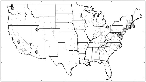
Table 1. FT-IR calibration, method testing, and FRM prediction samples distinguished by network, filter type, and field status (sampled vs. blank).
Figure 2. Illustration of the data available for CSN and FRM analysis as distinguished by sample network (CSN vs. FRM), study role (calibration vs. test set), or filter type (MTL vs. Whatman). Intersections symbolize the maximum number of TOR data available for FRM OC and EC evaluation. For example, of the 470 FRM Whatman filters collected, only 92 TOR samples are available for FRM OC and EC evaluation and for CSN calibration upper as shown in the upper left intersections in both diagrams (red–yellow). Another 46 TOR samples are available for FRM OC and EC evaluation and for CSN testing as shown in the upper right intersections in both diagrams (red–green). Field blanks are not considered here as no aerosol carbon is present.
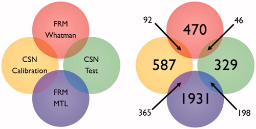
Figure 3. FRM OC predictions plotted against TOR OC reference concentrations. FT-IR OC predictions are first pooled (a = MTL + Whatman) and then distinguished by filter type (b = MTL, c = Whatman). Predicted OC areal densities are converted to the more familiar mass-concentrations (µg/m3) here.
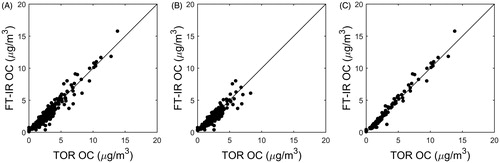
Table 2. FT-IR OC determined on FRM filters compared to the base case CSN OC from Weakley et al. (Citation2016).
Table 3. FT-IR EC determined on FRM filters compared to the base case CSN EC from Weakley et al. (Citation2018).
Table 4. Matched CSN and FRM OC and EC comparisons according to the scheme presented in .
Figure 4. TOR EC reference mass-concentrations plotted against FRM EC predictions. Predictions are pooled (a = MTL + Whatman) and then distinguished by filter type to aid comparison (b = MTL, c = Whatman). Predicted OC areal densities are converted to the more familiar mass-concentrations (µg/m3) here.
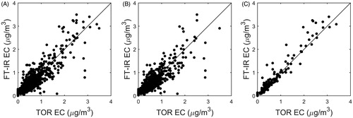
Figure 5. Average raw CSN Whatman (black) and FRM MTL (red) spectra plotted with their 5th and 95th percentiles (dashes; a). The most important wavenumbers used in the OC and EC calibrations, determined according to a variable importance in projection (VIP) score greater than one (Chong and Jun Citation2005), are indicated (as gray and blue lines), respectively. The processed Whatman and MTL spectra, in the two most analytically pertinent regions, are plotted to assess any connection between prediction bias and error variance (b, c).
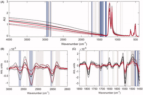
Figure 6. Predicted FT-IR OC in Fresno, CA samples (a) and Providence, RI samples (b). Samples validated against available TOR measurements as diamonds (gray) are distinguished from samples with no TOR data (“blinds”; bullets, black). A robust locally weighted error sum-of-squares (LOWESS) smoother was used to estimate the trend line in each series from validated data.
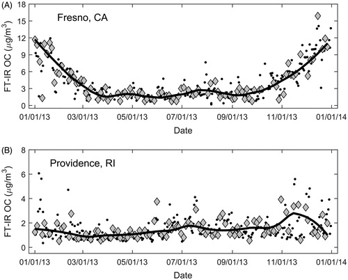
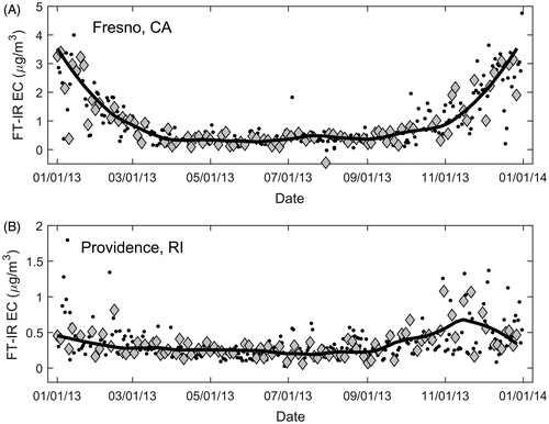
Figure 7. Predicted FT-IR EC in Fresno, CA samples (a) and Providence, RI samples (b). Samples validated against available TOR measurements as diamonds (gray) are distinguished from samples with no TOR data (“blinds”; bullets, black).