Figures & data
Figure 1. Geometry of the TSI Model 3081A long-column DMA (a) and the two-dimensional classification region (b). Details, such as the sheath in connection and the high voltage supply connection are omitted in (a), but the dimensions of the flow passages are derived directly from data by TSI, Inc., or measured in our laboratory.
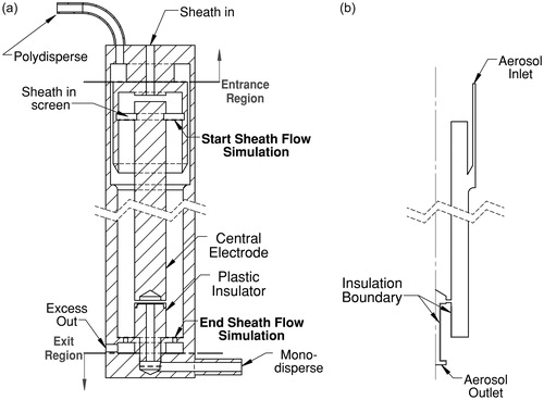
Table 1. Operation parameters of the scanning DMA.
Figure 2. Magnitude of fluid flow velocity and electric potential within the classification region: (a) flow field in the upper region; (b) flow field in the lower region; (c) electric field in the upper region; (d) electric field in the lower region. Note that the color scales in (a) and (b) are different. The white lines in (a) and (b) represent the fluid flow streamlines, and those in (c) and (d) are the electric field lines. The adverse electric potential gradient region is labeled in (d).
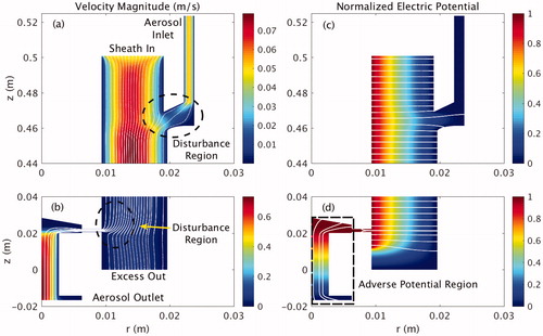
Figure 3. Particle trajectories within the DMA (a) entrance region, (b) exit region, (c) extended classification region for the actual DMA geometry, and (d) the idealized, parallel-flow classification region for 147 nm particles; the values of the length L, inner radius R1, and outer radius R2 are given in . The width of the aerosol sample incoming flow and classified sample outlet flow in the parallel-flow model are determined by the fraction of the total flow that corresponds to the corresponding limiting streamline.
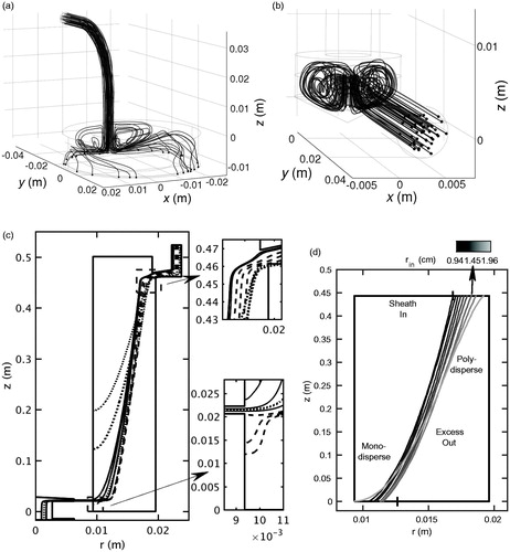
Figure 4. Spatial distribution of particles exiting the aerosol outlet of the DMA classification region. Data are fitted with a 3-term Gaussian model, , where
, and
are the fitting parameters.
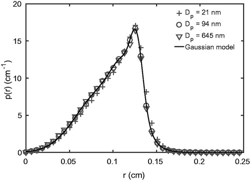
Figure 5. Scanning transfer functions for 24.5 nm particles through the real DMA geometry as determined using the indicated simulation time steps based for a ramp time of s.
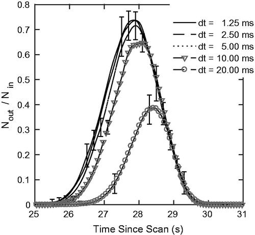
Figure 6. Penetration efficiency through the DMA entrance region as a function of particle diameter for an aerosol flow rate of LPM.
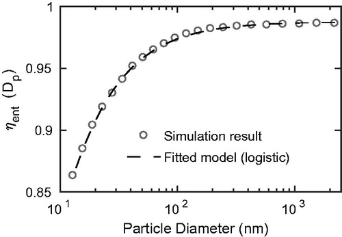
Figure 7. (a) Penetration distribution through the DMA exit region as a function of particle diameter and elapsed time; (b) the time variation of the penetration for 13, 34, and 2,204 nm particles; (c) cumulative particle penetration efficiency as a function of particle diameter; (d) mean residence time through the DMA exit region as a function of particle diameter.
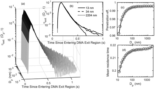
Figure 8. Temporal distributions of entrance and exit times for singly charged 147 nm particles that are successfully transmitted through the DMA classification region for the geometric-DMA (G-DMA) model, or through the classification region of the parallel-laminar-flow (PFDMA-L) model. Ramp times for both upscan (a) and downscan (b) was = 45 s (
= 6.94 s). The voltage was held constant for 20 s before the start of each scan (up or down).
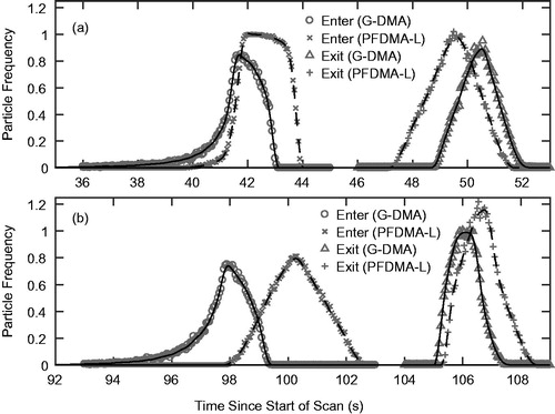
Figure 9. Up-scan transfer functions for 147 nm particles with a ramp time of , 20, 45, 90, and 240 s (corresponding to
, 3.08, 6.94, 13.9, and 37.0 s) for the geometric-DMA (G-DMA), parallel-laminar-flow (PFDMA-L) and parallel-plug-flow (PFDMA-P) models as a function of the classifier exit time. The static-DMA model uses the constant-voltage transfer function, as in the PFDMA-P model, but evaluates the transfer function at the time at which particles exit the DMA.
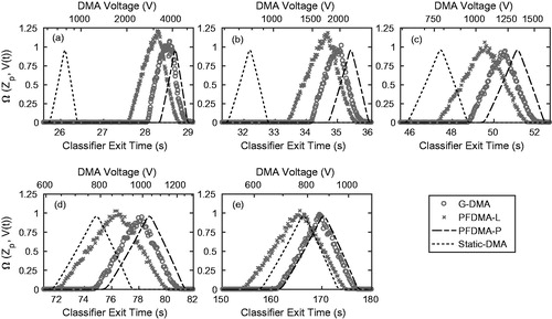
Figure 10. Down-scan transfer functions for 147 nm particles with ramping time = 10, 20, 45, 90, and 240 s (corresponding to
= 1.54, 3.08, 6.94, 13.87, and 37.00 s) for the geometric-DMA (G-DMA), parallel-laminar-flow (PFDMA-L), parallel-plug-flow (PFDMA-P), and static DMA models.
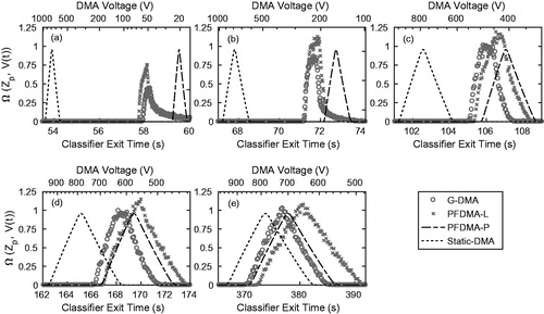
Figure 11. Scanning DMA transfer functions for singly charged particles, with electric mobility equivalent diameters ranging from 15.8 to 1130 nm. Scattered dots represent the raw data from the simulations, while the solid lines are the result obtained by applying locally weighted scatterplot smoothing (LOESS) to the raw data.
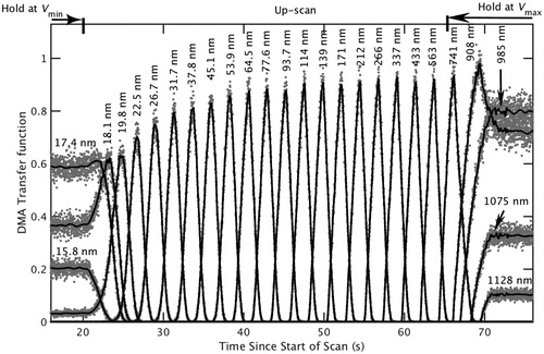
Figure 12. The scanning DMA transfer function as a function of the time-in-scan and the inverse particle electrical mobility. The inset (a) shows the transfer function during the transition from the low-voltage holding period to the ramp, while inset (b) shows the transfer function for particles whose transit is fully within the ramp.
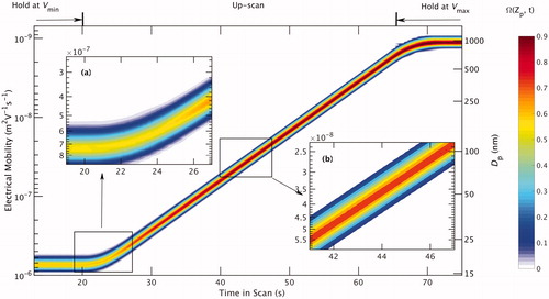
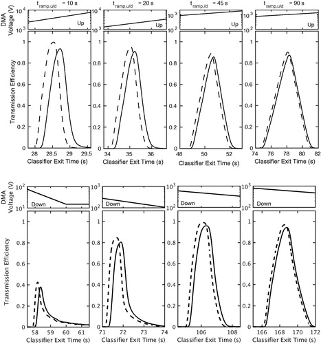
Figure 13. Transfer functions of the classification region (dashed line) and that of the complete DMA (including entrance and exit regions, solid line) for up-scan (upper panel) and down-scan (lower panel) operation for = 10, 20, 45, 90 s (corresponding to
= 1.54, 3.08, 6.94, 13.87 s).