Calibration of a particle mass spectrometer using polydispersed aerosol particles

Figures & data

Figure 1. (a) Schematic diagram and (b) operation procedure of the calibration method proposed in this study. The main components include an aerosol atomizer with an air compressor, diffusion dryer, and flow controllers for particle generation and dilution (the compressor and flow controllers are not shown).

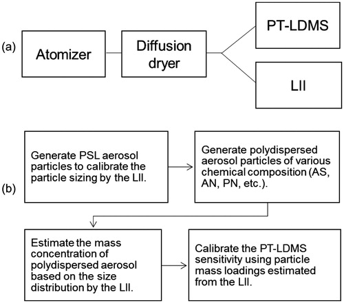
Figure 2. Pulse height distributions of LS signals of PSL (shaded), ammonium sulfate (AS, solid), and potassium nitrate (PN, dashed) particles classified by a DMA at a mobility diameter of 254 nm.

Figure 3. (a) Number size distribution of polydispersed AS particles measured by the LS method (solid sticks) and SMPS (shaded line). The arrows indicate “dip” size bins near the boundary of the detectors. The dashed line represents the lognormal fitting for the SMPS data. (b) Volume size distributions of polydispersed AS particles measured by the LS method (solid sticks) and SMPS (shaded line). The dashed line represents the lognormal fitting for the LS data. The “dip” size bins were excluded from the plot and fitting.

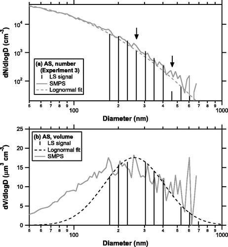
Table 1. Comparison of total volume concentrations between the LS method and SMPS.^a

	Ammonium sulfate (AS)	Potassium nitrate (PN)
Experiment 1	1.00 ± 0.05	1.11 ± 0.06
Experiment 2	0.93 ± 0.12	0.85 ± 0.04
Experiment 3	0.87 ± 0.15	0.78 ± 0.08

^a Average ratio of total volume concentrations of polydispersed aerosol particles derived from the LS method to that from the SMPS. The error represents one standard deviation.

Figure 4. Temporal profiles of ion signals at a mass-to-charge (m/z) ratio of 48 obtained for AS particles during experiment 3. The shaded and solid lines represent data from monodisperse (sulfate mass loadings of 12.7 ng) and polydisperse (11.3 ng) tests, respectively. The dashed line represents data from zero air (particle-free air).

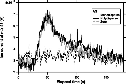
Figure 5. (a) Scatterplots of the integrated ion signal at m/z 48 for AS particles versus accumulated mass of SO₄²⁻ obtained from the conventional (monodisperse) and new (polydisperse) methods for experiments 1–3. The slope of the solid line (as indicated by the number on the top-right corner) represents the average sensitivity (pC ng⁻¹) of the conventional method. Error bars (one standard deviation) are shown for selected data points. (b) Same as (a) but for PN particles.

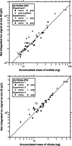
Table 2. Comparison of the MS sensitivity between the conventional and new methods.^a

	Sulfate (SO4^2−) from AS	Nitrate (NO3^−) from PN
Experiment 1	0.93 ± 0.15	0.91 ± 0.07
Experiment 2	1.03 ± 0.12	0.72 ± 0.04
Experiment 3	0.78 ± 0.08	0.83 ± 0.07

^a Ratio of the average sensitivity from the conventional method (mono-S_m/z) to that from the new method (poly-S_m/z). The error represents one standard deviation.