Multiple scattering correction factor estimation for aethalometer aerosol absorption coefficient measurement

Figures & data

Table 1. Instrument setup for ${\sigma }_{ap}$ measurements during CAPMEX and at GSN, LLN, and ALT.

Station	Period	Aethalometer^a (Filter-based optical)	PASS-3^b (Photoacoustic)	CLAP^c (Filter-based optical)
GSN (CAPMEX)	Aug.–Sep. 2008	No imposed RH, size cut	No imposed RH, size cut	NA^d
GSN	Jan. 2012–Dec., 2014	No imposed size cut RH < 40%	NA	10 μm size cut RH < 40%
LLN	Jan.–Dec., 2013
ALT	Sep. 2014–May, 2015

^a Aethalometer: 370, 470, 520, 590, 660, 880, and 950 nm.

^b PASS-3: 405, 532, and 781 nm.

^c CLAP: 467, 528, and 652 nm.

^d NA: Not Available.

Figure 1. Comparison between ${\sigma }_{ap}^{flc}$ and ${\sigma }_{ap}^{\mathit{\text{PASS}}3}$ during CAPMEX (dashed line (black) is the LRL; color scale indicates the occurrence).

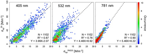
Table 2. Results of $C_{ref}$ determination during CAPMEX.

	405 nm	532 nm	781 nm
LRL	$y=3.99x-2.07$	$y=4.48x+6.92$	$y=5.46x+6.22$
SEa^a	0.04	0.07	0.05
SEb^b	0.48	0.46	0.18
$C_{ref}^{W03}$	3.67 ± 1.25^c	5.38 ± 2.73	7.11 ± 1.82
$C_{ref}^{LRL}$	3.99 ± 1.33	4.48 ± 2.32	5.46 ± 1.66
N		1102

^a SE_a: Standard Error of LRL slope.

^b SE_b: Standard Error of LRL intercept.

^c Mean ± standard deviation.

Figure 2. Box-whisker plot of (a) ${\mathit{C}}_{\mathit{r}\mathit{e}\mathit{f}}^{\mathit{W}03}$ and (b) ${\mathit{C}}_{\mathit{r}\mathit{e}\mathit{f}}^{\mathit{L}\mathit{R}\mathit{L}}$ segmented by percentiles of ${\mathit{\sigma }}_{\mathit{a}\mathit{p}}^{\mathit{P}\mathit{A}\mathit{S}\mathit{S}3}$ (bottom and top whiskers represent the 5^th and 95^th percentiles; horizontal lines of the box represent the 25^th, 50^th, and 75^th percentiles of ${\mathit{C}}_{\mathit{r}\mathit{e}\mathit{f}}$; dashed line (green) represents ${\mathit{C}}_{\mathit{r}\mathit{e}\mathit{f}}$; cross (red) represents the average value of each percentile of ${\mathit{\sigma }}_{\mathit{a}\mathit{p}}^{\mathit{P}\mathit{A}\mathit{S}\mathit{S}3}$; 0–10 on the x-axis represents the interval between the 0 and 10^th percentile of ${\mathit{\sigma }}_{\mathit{a}\mathit{p}}^{\mathit{P}\mathit{A}\mathit{S}\mathit{S}3}$). Numbers in parentheses in x-axis are the range of ${\mathit{\sigma }}_{\mathit{a}\mathit{p}}$ in each bin (unit in Mm⁻¹).

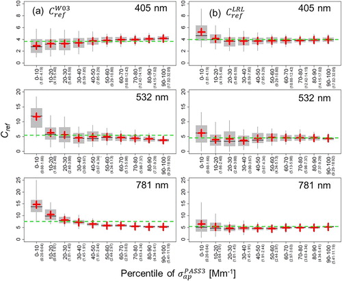
Table 3. ${\sigma }_{ap}^{\mathit{\text{PASS}}3}$-segmented $C_{ref}$ and their percentage difference from the unsegmented average of $C_{ref}$ during CAPMEX.

Percentile of ${\sigma }_{ap}^{\mathit{\text{PASS}}3}$		0–10	10–20	20–30	30–40	40–50	50–60	60–70	70–80	80–90	90–100	Total $C_{ref}$ (0–100)
Segmented $C_{ref}^{W03}$	405 nm	2.92	3.29	3.28	3.42	3.70	3.83	3.93	3.92	4.06	4.15	3.67
	532 nm	11.89	6.38	5.69	4.69	5.04	5.06	4.76	4.57	4.34	3.96	5.38
	781 nm	14.68	10.47	8.19	7.23	6.43	5.83	5.86	5.51	5.27	5.25	7.11
Difference from total $C_{ref}^{W03}$ [%]	405 nm	˗20.4	˗10.4	˗10.6	˗6.8	0.8	4.4	7.1	6.8	10.6	13.1	NA^a
	532 nm	121.0	18.6	5.9	˗12.8	˗6.2	˗5.8	˗11.3	˗14.9	˗19.3	˗26.5	NA
	781 nm	106.5	47.2	15.2	1.7	˗9.5	˗18.0	˗17.5	˗22.5	˗25.9	˗26.1	NA
Segmented $C_{ref}^{LRL}$	405 nm	4.11	3.72	3.72	3.73	3.78	3.82	3.79	3.91	3.95	4.11	3.99
	532 nm	6.13	3.92	4.16	3.61	4.31	4.62	4.53	4.54	4.50	4.35	4.48
	781 nm	6.83	5.71	5.05	5.18	5.13	4.96	5.34	5.34	5.37	5.69	5.46
Difference from total $C_{ref}^{LRL}$ [%]	405 nm	3.0	˗6.7	˗6.8	˗6.6	˗5.3	˗4.3	˗5.0	˗1.9	˗0.8	3.0	NA
	532 nm	36.8	˗12.5	˗7.14	˗19.4	˗3.8	3.1	1.1	1.3	0.4	˗2.9	NA
	781 nm	25.1	4.6	˗7.5	˗5.1	˗6.0	˗9.2	˗2.2	˗2.2	˗1.6	4.2	NA

^a NA: Not Available.

Figure 3. ${\mathit{C}}_{\mathit{r}\mathit{e}\mathit{f}}$ values from previous studies and those determined in this study (black: ${\mathit{C}}_{\mathit{r}\mathit{e}\mathit{f}}$ using a filter-free instrument and laboratory-generated/fresh soot; blue: ${\mathit{C}}_{\mathit{r}\mathit{e}\mathit{f}}$ using a filter-based optical instrument and ambient/coated aerosols; red: ${\mathit{C}}_{\mathit{r}\mathit{e}\mathit{f}}$ using a filter-free instrument and ambient/coated aerosols).

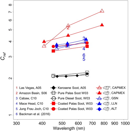
Table 4. Results of the comparison between ${\sigma }_{ap}^{W03}$, ${\sigma }_{ap}^{LRL}$, and ${\sigma }_{ap}^{\mathit{\text{CLAP}}}$ at GSN, LLN, and ALT.

		${\sigma }_{ap}$ [Mm^-1]^a			BD [Mm^-1]^b			RMSD [Mm^-1]^c			N
		467 nm	528 nm	652 nm	467 nm	528 nm	652 nm	467 nm	528 nm	652 nm
GSN	${\sigma }_{ap}^{W03}$	7.51 ± 5.49	5.92 ± 4.35	4.00 ± 2.91	˗ 0.25	˗ 0.81	˗ 1.20	1.35	1.27	1.34	13,662
	${\sigma }_{ap}^{LRL}$	7.45 ± 5.44	6.27 ± 4.60	4.73 ± 3.44	˗ 0.31	˗ 0.46	˗ 0.47	1.35	1.17	0.93
	${\sigma }_{ap}^{\mathit{\text{CLAP}}}$	7.76 ± 6.11	6.73 ± 5.28	5.20 ± 4.07	NA^d	NA	NA	NA	NA	NA
LLN	${\sigma }_{ap}^{W03}$	3.61 ± 5.13	2.84 ± 4.10	2.07 ± 2.81	˗ 0.07	˗ 0.34	˗ 0.51	0.65	0.64	0.69	4,151
	${\sigma }_{ap}^{LRL}$	3.58 ± 5.09	3.00 ± 4.33	2.38 ± 3.19	˗ 0.10	˗ 0.18	˗ 0.20	0.66	0.59	0.52
	${\sigma }_{ap}^{\mathit{\text{CLAP}}}$	3.68 ± 5.60	3.18 ± 4.91	2.58 ± 3.82	NA	NA	NA	NA	NA	NA
ALT	${\sigma }_{ap}^{W03}$	0.57 ± 0.41	0.45 ± 0.32	0.31 ± 0.22	˗ 0.01	˗ 0.07	˗ 0.10	0.10	0.09	0.12	4,431
	${\sigma }_{ap}^{LRL}$	0.56 ± 0.41	0.47 ± 0.34	0.36 ± 0.26	˗ 0.02	˗ 0.04	˗ 0.05	0.11	0.09	0.08
	${\sigma }_{ap}^{\mathit{\text{CLAP}}}$	0.58 ± 0.46	0.52 ± 0.40	0.40 ± 0.32	NA	NA	NA	NA	NA	NA

^aMean ± standard deviation.

^bBD = $\frac{1}{N}$.${\sum }_i^N\left({\sigma }_{ap,i}-{\sigma }_{ap,i}^{\mathit{\text{CLAP}}}\right)$

^cRMSD = $\frac{1}{N}$.${\sum }_i^N\sqrt{{\left({\sigma }_{ap}-{\sigma }_{ap}^{\mathit{\text{CLAP}}}\right)}^2}$

^dNA: Not Available.

Figure 4. Comparisons of aethalometer ${\mathit{\sigma }}_{\mathit{a}\mathit{p}}$ with ${\mathit{\sigma }}_{\mathit{a}\mathit{p}}^{\mathit{C}\mathit{L}\mathit{A}\mathit{P}}$. (a) ${\mathit{\sigma }}_{\mathit{a}\mathit{p}}^{\mathit{W}03}$ and (b) ${\mathit{\sigma }}_{\mathit{a}\mathit{p}}^{\mathit{L}\mathit{R}\mathit{L}}$ at GSN, (c) ${\mathit{\sigma }}_{\mathit{a}\mathit{p}}^{\mathit{W}03}$ and (d) ${\mathit{\sigma }}_{\mathit{a}\mathit{p}}^{\mathit{L}\mathit{R}\mathit{L}}$ at LLN, and (e) ${\mathit{\sigma }}_{\mathit{a}\mathit{p}}^{\mathit{W}03}$ and (f) ${\mathit{\sigma }}_{\mathit{a}\mathit{p}}^{\mathit{L}\mathit{R}\mathit{L}}$ at ALT (black and gray dashed lines are the LRL and 1:1 line, respectively; color scale represents the occurrence).

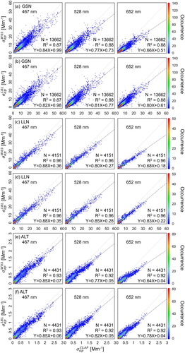
Figure 5. Frequency distributions of $\Delta {\sigma }_{ap}$ [= aethalometer ${\sigma }_{ap}-{\sigma }_{ap}^{\mathit{\text{CLAP}}}$] at (a) GSN, (b) LLN, and (c) ALT. Solid lines indicate the distributions of $\Delta {\sigma }_{ap}$ (${\sigma }_{ap}^{W03}$ is black; ${\sigma }_{ap}^{LRL}$ is red; vertical dashed line is the period average).

Figure 6. SSA retrieved at GSN, LLN, and ALT. SSA using ${\sigma }_{ap}^{W03}$, ${\sigma }_{ap}^{LRL}$, and ${\sigma }_{ap}^{\mathit{\text{CLAP}}}$ are denoted as black, red, and green, respectively (${\sigma }_{sp}$ is identical at each station).

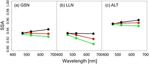
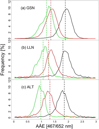
Figure 7. Frequency distributions of AÅE at (a) GSN, (b) LLN, and (c) ALT. Solid line is the distribution of ${\sigma }_{ap}^{W03}$ (black/right), ${\sigma }_{ap}^{LRL}$ (red/center), and ${\sigma }_{ap}^{\mathit{\text{CLAP}}}$ (green/left). Vertical dashed line is the average value.