High potential, near free molecular regime Coulombic collisions in aerosols and dusty plasmas

Figures & data

Figure 1. Histograms of $w$ inferred from Langevin simulations are shown for ${\Psi }_E=0,\mathrm{ }\frac{3}{2},\mathrm{ }7,\mathrm{ }60\mathrm{ }$for ${Kn}_D={10}^{-2},\mathrm{ }{10}^0,\mathrm{ }{10}^2.$ The gray bars represent the normalized counts $\mathrm{pdf}\left(w\right)$ of $w=\log \left(\frac{H\left({Kn}_D,{\Psi }_E\right)}{H_{HS}\left({Kn}_D\right)}\right)$ and the solid black line is the Gumbel distribution function (Equation (9)(9) $$\mathrm{pdf}\left(w\right)=e^{-(w-\mu )}{e}^{-e^{-(w-\mu )}}.$$(9) ) with the corresponding value of location parameter $\mu$ fitted for each case.

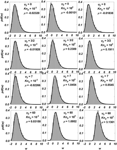
Figure 2. Fitted values of the location parameter $\mu$ for ${\Psi }_E=\frac{3}{2},7,\mathrm{ }30,\mathrm{ }60$ for ${Kn}_D={10}^{-2}-2000$ shown as data points. The corresponding fit for $\mu$ (Equation (11)(11) $$\mu \left({Kn}_D,{\Psi }_E\right)=\frac{C}{A}{\left(1+k\frac{\log {Kn}_D-B}{A}\right)}^{-\frac{1}{k}-1}\exp \left({-\left(1+k\frac{\log {Kn}_D-B}{A}\right)}^{-\frac{1}{k}}\right),\mathrm{ }k\ne 0.$$(11) ) is shown as dashed lines of the same color.

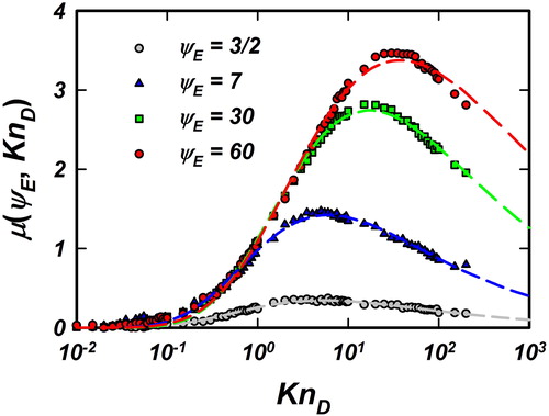
Figure 3. (a) Langevin-inferred $H$ (referred to as $H_{\mathrm{Langevin}}$) and prediction of Equation (10)(10) $$H({Kn}_D,{\Psi }_E)=e^{\mathrm{\mu }}{H}_{\mathit{HS}}\left({Kn}_D\right).$$(10) (dashed lines with the same color as the symbols) are plotted as a function of ${Kn}_D$ for ${\Psi }_E=\frac{3}{2},7,\mathrm{ }30,\mathrm{ }60.$ Also shown are the infinitely collisional (Equation (6a)(6a) $${Kn}_D\to 0:\mathrm{ }H=4\pi {Kn}_D^2,$$(6a) ) and collisionless (Equation (6b)(6b) $${Kn}_D\to \mathrm{\infty }:\mathrm{ }H=\sqrt{8\pi }{Kn}_D.$$(6b) ) limits as black dashed lines. (b) Plot showing the % difference between the prediction of Equation (10)(10) $$H({Kn}_D,{\Psi }_E)=e^{\mathrm{\mu }}{H}_{\mathit{HS}}\left({Kn}_D\right).$$(10) and $H_{\mathrm{Langevin}}$ defined as $\frac{H_{\mathrm{model}}-H_{\mathrm{Langevin}}}{H_{\mathrm{Langevin}}}\left(\mathrm{\%}\right).$ The same symbols are used in both plots to denote different values of ${\Psi }_E.$ Reference lines at $\pm 10\mathrm{\%}$ are included to guide the eye. A compilation of more the datasets and their deviations from predictions of Equation (10)(10) $$H({Kn}_D,{\Psi }_E)=e^{\mathrm{\mu }}{H}_{\mathit{HS}}\left({Kn}_D\right).$$(10) are provided in Figure S3, SI.

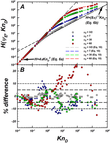
Figure 4. Plot showing the Langevin-inferred $H$ (referred to as $H_{\mathrm{Langevin}}$) for ${\Psi }_E=7,\mathrm{ }30,\mathrm{ }60.$ Panels (a–c) present $H_{\mathrm{Langevin}}$ for $S_D={10}^{-1},\mathrm{ }{10}^1,\mathrm{ }{10}^2,\mathrm{ }{10}^3$ as data points. The continuum limit (Equation (6a)(6a) $${Kn}_D\to 0:\mathrm{ }H=4\pi {Kn}_D^2,$$(6a) ) and free molecular limit (Equation (6b)(6b) $${Kn}_D\to \mathrm{\infty }:\mathrm{ }H=\sqrt{8\pi }{Kn}_D.$$(6b) ) are shown as black dotted lines. Also shown is the hard sphere fit (Equation (8)(8) $$H({Kn}_D,{\Psi }_E=0)=H_{\mathit{HS}}\left({Kn}_D\right)=\frac{4\pi {Kn}_D^2+25.836{Kn}_D^3+\sqrt{8\pi }{Kn}_D\left(11.211{Kn}_D^3\right)}{1+3.502{Kn}_D+7.211{Kn}_D^2+11.211{Kn}_D^3}.$$(8) ) and the unscreened Coulomb model (Equation (10)(10) $$H({Kn}_D,{\Psi }_E)=e^{\mathrm{\mu }}{H}_{\mathit{HS}}\left({Kn}_D\right).$$(10) ). The common legend for panels (a–c) is given in panel (b). Panels (d–f) plot the comparison of the difference between the Langevin-inferred $H$ (referred to as $H_{\mathrm{Langevin}}$) and (1) the prediction of the hard sphere fit (referred to as $H_{\mathrm{Eq}.8}$) for $S_D={10}^{-1}$ shown as blue triangles and (2) the prediction of Coulomb model (referred to as $H_{\mathrm{Eq}.10}$) for $S_D={10}^3$ shown as green circles. Reference lines for denoting difference levels of $\pm 10\mathrm{\%}$ and $\pm 20\mathrm{\%}$ are shown to guide the eye. The common legend for panels (d–f) is given at the bottom.

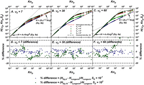
Figure 5. Langevin-inferred $H$ (referred to as $H_{\mathrm{Langevin}}$ shown as green circles with black outline) and the predictions of various models considered for evaluation are plotted as a function of ${\mathit{Kn}}_D$ for ${\Psi }_E=\frac{3}{2},7,\mathrm{ }30,\mathrm{ }60.$ In each panel, the predictions of the unscreened Coulomb ($S_D=\mathrm{\infty }$) model (Equation (10)(10) $$H({Kn}_D,{\Psi }_E)=e^{\mathrm{\mu }}{H}_{\mathit{HS}}\left({Kn}_D\right).$$(10) , blue dashed line), D’Yachkov et al. (2007) in orange, Gatti and Kortshagen (2008) in pink, Gopalakrishnan and Hogan (2012) in dark green, and Zobnin et al. (2008) in red are shown. Also shown are the infinitely collisional (Equation (6a)(6a) $${Kn}_D\to 0:\mathrm{ }H=4\pi {Kn}_D^2,$$(6a) ) and collision-less (Equation (6b)(6b) $${Kn}_D\to \mathrm{\infty }:\mathrm{ }H=\sqrt{8\pi }{Kn}_D.$$(6b) ) limits as dashed black lines. For comparison of the difference between model predictions and $H_{\mathrm{Langevin}},$ see Figure 6.

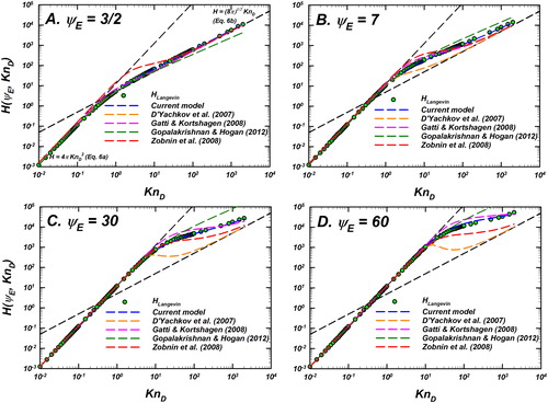
Figure 6. Comparison of the difference between the Langevin-inferred $H$ (referred to as $H_{\mathrm{Langevin}}$) and the prediction of various models as noted in the legend for ${\Psi }_E=\frac{3}{2},\mathrm{ }7,\mathrm{ }30,\mathrm{ }60$ as a function of ${Kn}_D.$ Differences of the models considered are shown as dashed lines including the current model (Equation (10)(10) $$H({Kn}_D,{\Psi }_E)=e^{\mathrm{\mu }}{H}_{\mathit{HS}}\left({Kn}_D\right).$$(10) with $S_D=\mathrm{\infty }$) in blue, D’Yachkov et al. (2007) in orange, Gatti and Kortshagen (2008) in pink, Gopalakrishnan and Hogan (2012) in dark green, and Zobnin et al. (2008) in red. The y-axis shows the % difference between the predictions of each model and $H_{\mathrm{Langevin}}.$ % difference is defined as $\frac{H_{\mathrm{model}}-H_{\mathrm{Langevin}}}{H_{\mathrm{Langevin}}}\left(\mathrm{\%}\right).$ Reference lines for denoting difference levels of $\pm 10\mathrm{\%}$ and $\pm 20\mathrm{\%}$ are shown to guide the eye. This plot is to be read in conjunction with Figure 5.

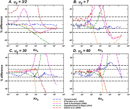
Figure 7. Langevin-inferred $H$ (referred to as $H_{\mathrm{Langevin}}$ shown as green circles with black outline) and the predictions of various models considered for evaluation are plotted as a function of ${Kn}_D$ for ${\Psi }_E=10,\mathrm{ }30,\mathrm{ }50,\mathrm{ }60$ and a fixed $S_D=10.$ In each panel, the predictions of the unscreened Coulomb model (Equation (10)(10) $$H({Kn}_D,{\Psi }_E)=e^{\mathrm{\mu }}{H}_{\mathit{HS}}\left({Kn}_D\right).$$(10) , blue dashed line), Gatti and Kortshagen (2008) in pink, Zobnin et al. (2008) in red and Hutchinson and Patacchini (2007) in gray are shown. Also shown are the infinitely collisional (Equation (6a)(6a) $${Kn}_D\to 0:\mathrm{ }H=4\pi {Kn}_D^2,$$(6a) ) and collision-less (Equation (6b)(6b) $${Kn}_D\to \mathrm{\infty }:\mathrm{ }H=\sqrt{8\pi }{Kn}_D.$$(6b) ) limits as black dashed lines. For comparison of the difference between model predictions and $H_{\mathrm{Langevin}},$ see Figure 8.

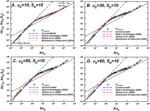
Figure 8. Comparison of the difference between the Langevin-inferred $H$ (referred to as $H_{\mathrm{Langevin}}$) and the prediction of various models as noted in the legend for ${\Psi }_E=10,\mathrm{ }30,\mathrm{ }50,\mathrm{ }60$ and a fixed $S_D=10.$ Differences of the models considered are shown as dashed lines including the current model (Equation (10)(10) $$H({Kn}_D,{\Psi }_E)=e^{\mathrm{\mu }}{H}_{\mathit{HS}}\left({Kn}_D\right).$$(10) ) in blue, Gatti and Kortshagen (2008) in pink, Zobnin et al. (2008) in red, and Hutchinson and Patacchini (2007) in gray. The y-axis shows the % difference between the predictions of each model and $H_{\mathrm{Langevin}}.$ % difference is defined as $\frac{H_{\mathrm{model}}-H_{\mathrm{Langevin}}}{H_{\mathrm{Langevin}}}\left(\mathrm{\%}\right).$ Reference lines for denoting difference levels of $\pm 10\mathrm{\%}$ and $\pm 20\mathrm{\%}$ are shown to guide the eye. This plot is to be read in conjunction with Figure 7.

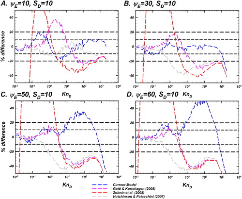
Figure 9. Langevin-inferred $H$ (referred to as $H_{\mathrm{Langevin}}$ shown as green circles with black outline) and the predictions of various models considered for evaluation are plotted as a function of ${Kn}_D$ for ${\Psi }_E=10,\mathrm{ }30,\mathrm{ }50,\mathrm{ }60$ and a fixed $S_D=100.$ In each panel, the predictions of the unscreened Coulomb model (Equation (10)(10) $$H({Kn}_D,{\Psi }_E)=e^{\mathrm{\mu }}{H}_{\mathit{HS}}\left({Kn}_D\right).$$(10) , blue dashed line), Gatti and Kortshagen (2008) in pink, Zobnin et al. (2008) in red, and Hutchinson and Patacchini (2007) in gray are shown. Also shown are the infinitely collisional (Equation (6a)(6a) $${Kn}_D\to 0:\mathrm{ }H=4\pi {Kn}_D^2,$$(6a) ) and collision-less (Equation (6b)(6b) $${Kn}_D\to \mathrm{\infty }:\mathrm{ }H=\sqrt{8\pi }{Kn}_D.$$(6b) ) limits as black dashed lines. For comparison of the difference between model predictions and $H_{\mathrm{Langevin}},$ see Figure 10.

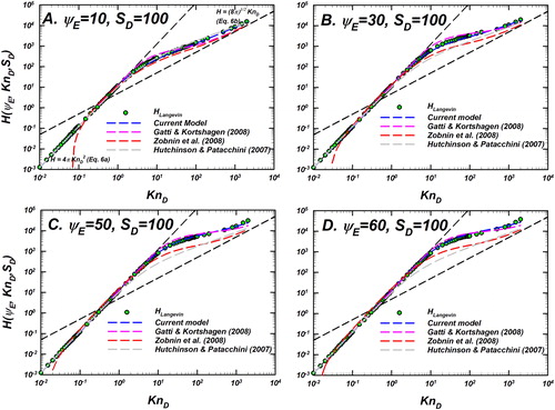
Figure 10. Comparison of the difference between the Langevin-inferred $H$ (referred to as $H_{\mathrm{Langevin}}$) and the prediction of various models as noted in the legend for ${\Psi }_E=10,\mathrm{ }30,\mathrm{ }50,\mathrm{ }60$ and a fixed $S_D=100.$ Differences of the models considered are shown as dashed lines including the current model (Equation (10)(10) $$H({Kn}_D,{\Psi }_E)=e^{\mathrm{\mu }}{H}_{\mathit{HS}}\left({Kn}_D\right).$$(10) ) in blue, Gatti and Kortshagen (2008) in pink, Zobnin et al. (2008) in red, and Hutchinson and Patacchini (2007) in gray. The y-axis shows the % difference between the predictions of each model and $H_{\mathrm{Langevin}}.$ % difference is defined as $\frac{H_{\mathrm{model}}-H_{\mathrm{Langevin}}}{H_{\mathrm{Langevin}}}\left(\mathrm{\%}\right).$ Reference lines for denoting difference levels of $\pm 10\mathrm{\%}$ and $\pm 20\mathrm{\%}$ are shown to guide the eye. This plot is to be read in conjunction with Figure 9.

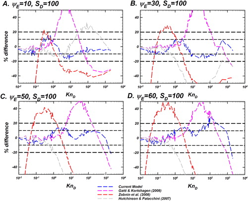
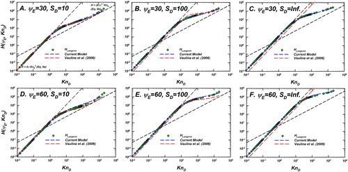
Figure 11. Langevin-inferred $H$ (referred to as $H_{\mathrm{Langevin}}$ shown as green circles with black outline) and the predictions of Langevin dynamics based models—the current model and the model of Vaulina, Repin, and Petrov (2006) are plotted as a function of ${\mathit{Kn}}_D$ for ${\Psi }_E=30,\mathrm{ }60$ and $S_D=10,\mathrm{ }100,\mathrm{ }\mathrm{\infty }.$ In each panel, the predictions of the current model (Equation (10)(10) $$H({Kn}_D,{\Psi }_E)=e^{\mathrm{\mu }}{H}_{\mathit{HS}}\left({Kn}_D\right).$$(10) , blue dashed line) and Vaulina, Repin, and Petrov (2006) (red dashed line) are shown. Also shown are the infinitely collisional (Equation (6a)(6a) $${Kn}_D\to 0:\mathrm{ }H=4\pi {Kn}_D^2,$$(6a) ) and collision-less (Equation (6b)(6b) $${Kn}_D\to \mathrm{\infty }:\mathrm{ }H=\sqrt{8\pi }{Kn}_D.$$(6b) ) limits as black dashed lines.

D’Yachkov, L. G., A. G. Khrapak, S. A. Khrapak, and G. Morfill. 2007. Model of grain charging in collisional plasmas accounting for collisionless layer. Phys. Plasmas 14 (4):042102.

 Web of Science ®Google Scholar

Gatti, M., and U. Kortshagen. 2008. Analytical model of particle charging in plasmas over a wide range of collisionality. Phys. Rev. E 78:046402. doi: 10.1103/PhysRevE.78.046402.

 Web of Science ®Google Scholar

Gopalakrishnan, R., and C. J. Hogan. 2012. Coulomb-influenced collisions in aerosols and dusty plasmas. Phys. Rev. E 85:026410.

 Web of Science ®Google Scholar

Zobnin, A. V., A. D. Usachev, O. F. Petrov, and V. E. Fortov. 2008. Ion current on a small spherical attractive probe in a weakly ionized plasma with ion-neutral collisions (kinetic approach). Phys. Plasmas 15 (4):043705. doi: 10.1063/1.2903052.

 Web of Science ®Google Scholar

Hutchinson, I. H., and L. Patacchini. 2007. Computation of the effect of neutral collisions on ion current to a floating sphere in a stationary plasma. Phys. Plasmas 14 (1):013505. doi: 10.1063/1.2431584.

 Web of Science ®Google Scholar

Vaulina, O. S., A. Y. Repin, and O. F. Petrov. 2006. Empirical approximation for the ion current to the surface of a dust grain in a weakly ionized gas-discharge plasma. Plasma Phys. Rep. 32 (6):485–488. doi: 10.1134/S1063780X06060055.

 Web of Science ®Google Scholar