Optimizing the performance of aerosol photoacoustic cells using a finite element model. Part 2: Application to a two-resonator cell

Figures & data

Figure 1. (a) Example data for PAS microphone response, using the PA cell design of Lack et al. (2006), over time during airborne measurements aboard the UK research aircraft (FAAM BAe-146), including measurements for sampling ambient aerosol particles and for where the sample was passed through a HEPA filter (background). Measurements were made above the South East Atlantic Ocean during flight C043 of the CLARIFY-2017 field campaign based at Ascension Island (Zuidema et al. 2016). For comparison, we show the variation in pressure associated with changes in altitude over the range 0–7.5 km. The plot also shows the interpolated pressure-dependent background, using a quadratic polynomial to relate the background response to pressure. (b) The standard error in PAS-measured α_abs associated with uncertainty in the interpolated background microphone response.

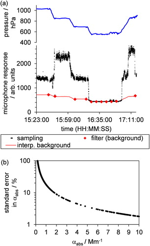
Figure 2. (a) The meshed geometry for the two-resonator cell with flat windows including two reflection symmetry planes; one parallel to the z-x plane through the center of the cell (longitudinal mirror plane) and one parallel to the z-y plane (transverse mirror plane). (b) The meshed geometry for the Brewster window cell. (c) Labeled dimensions for the Brewster window cell, with perspectives along the longitudinal and transverse mirror planes. Table 1 provides values for these dimensions. (d) For the Brewster window cell, the highlighted volumes indicate regions where periodic sample or window heating was applied.

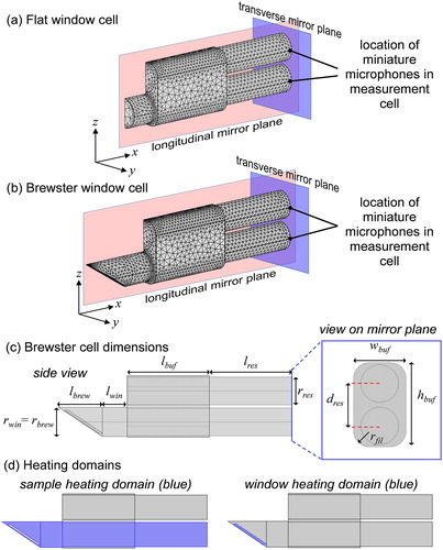
Table 1. Geometric parameters for the two-resonator PA cell.

Quantity	Description	Value
lres	Length of resonators	11.0 cm
rres	Radius of resonators	1.0 cm
dres	Separation of the lower and upper resonator centers	2.2 cm
lbuf	Length of buffer volumes	5.5 cm (lres/2)
hbuf	Height of buffer volumes	4.2 cm
wbuf	Width of buffer volumes	2.6 cm
rfil	Fillet radius for corners of buffer volumes	0.8 cm
lwin	Length of window volumes	1.0 cm
rwin	Radius of window volumes	1.0 cm
θB	Brewster angle for UV fused silica at optical wavelength of 660 nm	55°

Figure 3. Comparison of the eigenmode pressure distributions for the two-resonator cell with either (a) flat windows or (b) Brewster-angled windows.

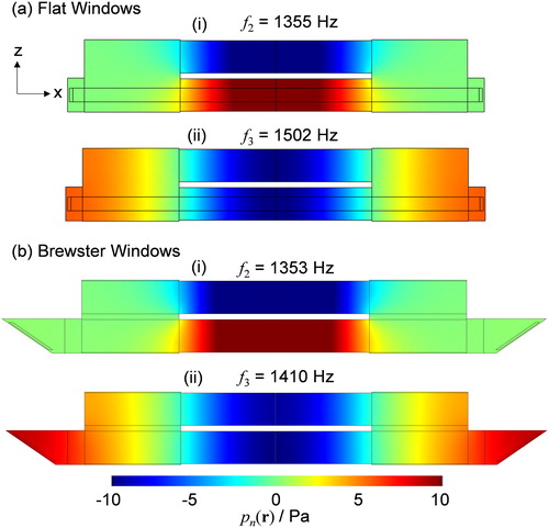
Figure 4. FEM predictions for the flat window cell of the frequency-dependent pressure responses $\left|p\left({\overrightarrow{\mathrm{r}}}_{\mathrm{M},\mathit{low}}\right)\right|$, $\left|p\left({\overrightarrow{\mathrm{r}}}_{\mathrm{M},\mathit{up}}\right)\right|,$ and $\left|p\left({\overrightarrow{\mathrm{r}}}_{\mathrm{M},\mathit{dif}}\right)\right|$ . Simulations are shown for the cases of (a) sample heating (α_sample = 5 Mm⁻¹) and (b) window heating (α_win = 0.1653 m⁻¹). We compare the sample heating simulations to measured data using speaker excitation, with measurements representing the mean response over five PA spectrometers.

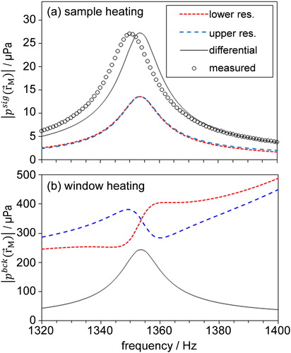
Figure 5. FEM predictions of microphone response for the Brewster window cell compared with measured data. (a) Simulations of $\left|p^{\mathit{sig}}\left({\overrightarrow{\mathrm{r}}}_{\mathrm{M}},\omega \right)\right|$ for the individual microphone and differential responses compared to measured differential operation data using speaker excitation. (b),(c),(d) Predictions of $\left|p^{\mathit{bck}}\left({\overrightarrow{\mathrm{r}}}_{\mathrm{M}},\omega \right)\right|$ (window heating) with the measured IA_bck for detection by the lower microphone, upper microphone, and differential response, respectively. Measured data are shown for four separate PA spectrometers using 405 nm (two spectrometers), 514 nm, or 658 nm laser excitation. The measured IA_bck has been normalized to scale from 0 to 1. The lines for the measured IA series are to guide the eye only.

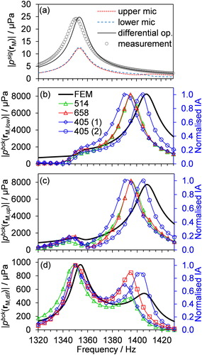
Figure 6. The eigenmode pressure distributions p_n($\overrightarrow{\mathrm{r}}$) for (a) the ring mode, and (b) the longitudinal mode with varying l_buf. The color scale range has been expanded to emphasize important variations in p_n($\overrightarrow{\mathrm{r}}$) with changing l_buf. In particular, the variation in p_n($\overrightarrow{\mathrm{r}}$) within the window volumes for the ring mode and the eigenmode pressure in the two resonator pipes for the longitudinal mode is emphasized.

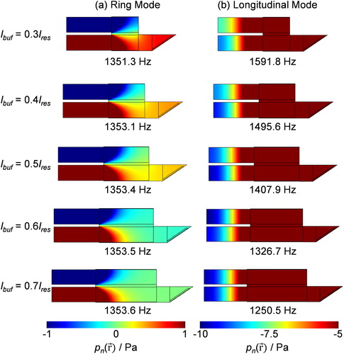
Figure 7. The FEM-predicted frequency dependence of (a) |p^sig(${\overrightarrow{\mathrm{r}}}_{M,\mathit{dif}})$| and (b) |p^bck(${\overrightarrow{\mathrm{r}}}_{M,\mathit{dif}})$| for values of l_buf in the range 0.1 l_res – 0.7 l_res in 0.1 l_res intervals. The legend indicates the $l_{\mathit{buf}}/l_{\mathit{res}}$ ratio for different series. (c) The variation in SBR with l_buf.

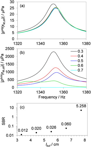
Figure 8. The variation in (a) |p^sig($\overrightarrow{\mathrm{r}}$ _M,dif, ω_n)|, (b) |p^bck($\overrightarrow{\mathrm{r}}$ _M,dif, ω_n)|, and (c) SBR with w_buf over the range 2.5–4.5 cm. Different data series are shown for the range of h_buf input to FEM simulations, from 4.5 cm to 6.0 cm in 0.5 cm steps. Lines are to guide the eye only.

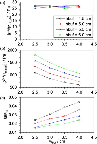
Figure 9. (a) The predicted SBR with variation in l_buf/l_res for the candidate two-resonator cell for which the total cell length is constrained to 22 cm, compared with the SBR variations presented in Figure 7. (b) Comparison of the predicted frequency-dependent differential amplified microphone responses for sample heating for the original (blue curve) and optimized (red curve) PA cells. (c) Same as (b) but for window heating excitation. The ring mode eigenfrequencies for the current (dashed blue line) and optimized (dashed red line) cells are indicated.

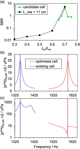
Table 2. Geometric parameters describing the optimized two-resonator PA cell.

Quantity	Value
lres	9.2 cm
rres	0.9 cm
dres	2.1 cm
lbuf	6.4 cm (0.7lres)
hbuf	4.1 cm
wbuf	2.6 cm
rfil	1.2 cm (0.9wbuf/2)
lwin	1.0 cm
rwin	1.0 cm
θB	55°

Figure 10. (a) For laser heating of the Brewster windows, the measured IA at the ring mode eigenfrequency for the original (old) and optimized (new) cells for laser wavelengths of 405 and 658 nm. The mean IA for ambient noise when the laser is off is also shown. (b) A time series in the measured IA for the optimized cell when the 658-nm laser is on or off. An indicative scale is shown on the right axis for absorption coefficient based on calibration of the cell using O₃.

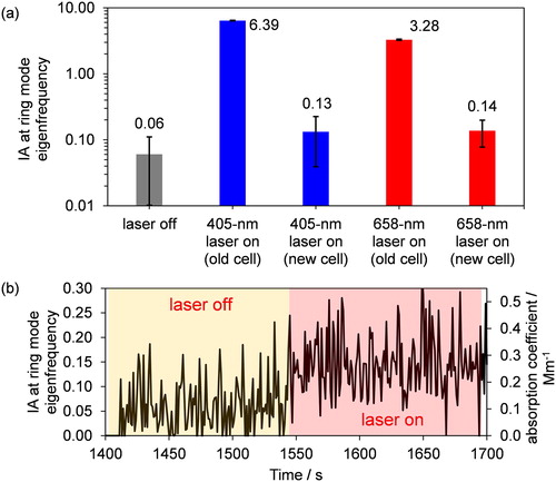
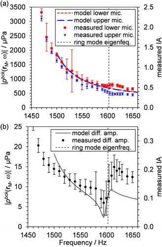
Figure 11. Comparison of FEM predictions of |p^bck($\overrightarrow{\mathrm{r}}$ _M, ω)| with measurements of microphone response (IA_bck) for the optimized cell for (a) lower and upper microphone responses, and (b) differential amplifier response. Error bars in (a) and (b) indicate one standard deviation in the measured IA_bck for 30 s of measurements.

Lack, D. A., E. R. Lovejoy, T. Baynard, A. Pettersson, and A. R. Ravishankara. 2006. Aerosol absorption measurement using photoacoustic spectroscopy: Sensitivity, calibration, and uncertainty developments. Aerosol Sci. Technol. 40 (9):697–708. doi: 10.1080/02786820600803917.

 Web of Science ®Google Scholar

Zuidema, P., J. Redemann, J. Haywood, R. Wood, S. Piketh, M. Hipondoka, and P. Formenti. 2016. Smoke and clouds above the southeast Atlantic: Upcoming field campaigns probe absorbing aerosol’s impact on climate. Bull. Amer. Meteor. Soc. 97 (7):1131–1135. doi: 10.1175/BAMS-D-15-00082.1.

 Web of Science ®Google Scholar

Data availability

For data related to this paper, please contact Michael I. Cotterell ([email protected]).