A semi-automated multi-endpoint reactive oxygen species activity analyzer (SAMERA) for measuring the oxidative potential of ambient PM_2.5 aqueous extracts

Figures & data

Figure 1. The system setup (a) and algorithm (b) of Semi-Automated Multi-Endpoint ROS Activity Analyzer (SAMERA).

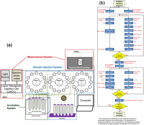
Figure 2. OP as a function of the concentration of positive controls: (a) OP^AA-SLF vs. Cu(II) concentrations; (b) OP^GSH-SLF vs. Cu(II) concentrations; (c) OP^OH-SLF vs. Fe(II) concentrations; (d) OP^DTT vs. PQ concentrations; (e) OP^OH-DTT vs. 5-H-1,4-NQ concentrations. The error bars represent the standard deviation of triplicate OP analysis.

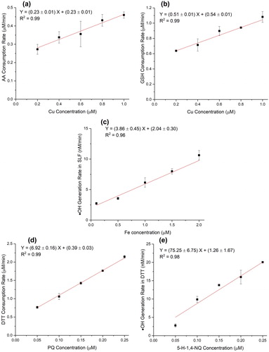
Figure 3. Comparison of manual operation (X axis) and automated system (Y axis) using four positive controls: (a) OP^AA-SLF of Cu(II); (b) OP^GSH-SLF of Cu(II); (c) OP^OH-SLF of Fe(II); (d) OP^DTT of PQ; (e) OP^OH-DTT of 5-H-1,4-NQ. The error bars on X and Y axes denote the standard deviation of triplicate OP analysis by both manual operation and automated system, respectively. The identity line is plotted as the dotted line.

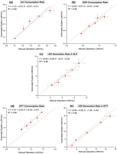
Figure 4. Comparison of manual operation (X axis) and automated system (Y axis) using ambient Hi-Vol filter samples (N = 9): (a) OP^AA-SLF; (b) OP^GSH-SLF; (c) OP^OH-SLF; (d) OP^DTT; (e) OP^OH-DTT. The identity line is plotted as the dotted line.

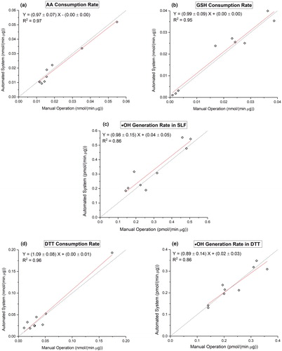
Table 1. The average blank levels and LOD of SAMERA for five OP endpoints as measured from both DI blanks and field blank filters.

Endpoint	Unit	DI blank		Filter blank filters
		Average	LOD	Average	LOD
OP^AA-SLF	µM/min	0.150	0.197	0.169	0.210
OP^GSH-SLF	µM/min	0.297	0.144	0.368	0.165
OP^OH-SLF	nM/min	3.390	1.824	4.570	3.633
OP^DTT	µM/min	0.496	0.060	0.651	0.065
OP^OH-DTT	nM/min	−0.463	0.634	−0.385	0.724

Table 2. Precision of SAMERA as obtained by multiple (N = 10) measurements of various standard chemicals.

Endpoint	Unit	Standard Chemical	Average	Standard Deviation	CoV (%)
OP^AA-SLF	µM/min	1 µM Cu(II)	0.405	0.033	8.11
OP^GSH-SLF	µM/min	1 µM Cu(II)	0.737	0.044	6.03
OP^OH-SLF	nM/min	2 µM Fe(II)	11.74	0.83	7.10
OP^DTT	µM/min	0.2 µM PQ	1.867	0.094	5.04
OP^OH-DTT	nM/min	0.2 µM 5-H-1,4-NQ	15.83	0.77	4.89

The concentration of the standard chemical refers to concentration in the reaction vial. CoV is the percentage ratio of the standard deviation to the average level.

Table 3. Precision of SAMERA as obtained by multiple (N = 10) measurements of an ambient PM_2.5 sample.

Endpoint	Unit	Average	Standard Deviation	CoV (%)
OP^AA-SLF	nmol/(min·µg)	0.0166	0.00196	11.87
OP^GSH-SLF	nmol/(min·µg)	0.0281	0.00221	7.89
OP^OH-SLF	nmol/(min·µg)	0.437	0.0462	10.56
OP^DTT	pmol/(min·µg)	0.0367	0.00387	10.52
OP^OH-DTT	pmol/(min·µg)	0.0489	0.00650	13.28

Figure 5. Mass and volume normalized OP of ambient PM_2.5 using the Hi-Vol samples collected from five sites in the Midwest US (N = 44): (a) OP^AA-SLF; (b) OP^GSH-SLF; (c) OP^OH-SLF; (d) OP^DTT; (e) OP^OH-DTT. Mass-normalized (OPm) and volume-normalized (OPv) of all samples are denoted by hollow and solid circles, respectively.

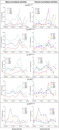
Table 4. Comparison of ambient PM2.5 OP obtained from SAMERA with those reported in the literatures.

Reference	PM size fraction (µm)	Levels	Location	Location type	Sample size
(a) OP^AA
Fang et al. (2016)^a	≤ 2.5	0.2 – 5.2 nmol·min^−1·m^−3	Southeast US	Urban and rural	483
Mudway et al. (2005)^b	≤ 2.5	0.012 ± 0.0001 nmol·min^−1·µg^−1	Eksaal, India	Biomass burning	3
Künzli et al. (2006)^b	≤ 2.5	0.0096 ± 0.0025 nmol·min^−1·µg^−1	19 European cities	Urban	716
Szigeti et al. (2016)^b^,^c	≤ 2.5	0.0017 – 0.04 nmol·min^−1·µg^−1	8 European cities	Urban	22
Godri et al. (2011)^b	1.0 – 1.9	0.0058 ± 0.0025 nmol·min-1·µg-1	London, United Kingdom	Urban	14
This study (OP^AA-SLF)	≤ 2.5	0.004 – 0.077 nmol·min^−1·µg^−1	Midwest US (5 sites)	Urban(4),rural(1)	54
		median: 0.012 nmol·min^−1·µg^−1
		0.044 – 0.745 nmol·min^−1·m^−3
		median: 0.160 nmol·min-1·m-3
(b) OP^GSH
Mudway et al. (2005)^b	≤ 2.5	0.0083 ± 0.0002 nmol·min^−1·µg^−1	Eksaal, India	Biomass burning	3
Künzli et al. (2006)^b	≤ 2.5	0.0041 ± 0.0017 nmol·min^−1·µg^−1	19 European cities	Urban	716
Szigeti et al. (2016)^b^,^c	≤ 2.5	0 – 0.0275 nmol·min^−1·µg^−1	8 European cities	Urban	22
Godri et al. (2011)^b	1.0 – 1.9	0.0042 ± 0.0033 nmol·min-1·µg-1	London, United Kingdom	Urban	14
This study (OP^GSH-SLF)	≤ 2.5	0.001 – 0.040 nmol·min^−1·µg^−1	Midwest US (5 sites)	Urban(4),rural(1)	54
		median: 0.010 nmol·min^−1·µg^−1
		0.008 – 0.463 nmol·min^−1·m^−3
		median: 0.100 nmol·min^−1·m^−3
(c) OP^OH-SLF
Vidrio et al. (2009)^d	≤ 2.5	0.253 ± 0.135 pmol·min^−1·µg^−1	Davis, CA	Urban	∼90
Ma et al. (2015)^d	≤ 2.5	0.092 ± 0.019 pmol·min-1·µg-1	Guangzhou, China	Urban	72
This study	≤ 2.5	0.085 – 0.967 pmol·min^−1·µg^−1	Midwest US (5 sites)	Urban(4),rural(1)	54
		median: 0.307 pmol·min^−1·µg^−1
		0.857 – 7.884 pmol·min^−1·m^−3
		median: 3.559 pmol·min-1·m-3
(d) OP^DTT
Fang et al. (2016)	≤ 2.5	0.15 – 0.43 nmol·min^−1·m^−3	Southeast US	Urban and rural	483
Xiong et al. (2017)	≤ 2.5	0.1 – 0.18 nmol·min^−1·m^−3	Urbana, IL	Urban	10
Verma et al. (2014)	≤ 2.5	0.018 – 0.055 nmol·min^−1·µg^−1	Atlanta area, GA	Urban, rural	483
Cho et al. (2005)	≤ 2.5	0.005 – 0.155 nmol·min^−1·µg^−1	Los Angeles basin, CA	Urban	11
Charrier et al. (2015)	≤ 2.5	0.02 – 0.061 nmol·min^−1·µg^−1	San Joaquin, CA	Urban, rural	6
Hu et al. (2008)	0.25 – 2.5	0.014 – 0.024 nmol·min-1·µg-1	Los Angeles harbor, CA	Urban	84
This study	≤ 2.5	0.004 – 0.193 nmol·min^−1·µg^−1	Midwest US (5 sites)	Urban(4),rural(1)	54
		median: 0.014 nmol·min^−1·µg^−1
		0.041 – 1.282 nmol·min^−1·m^−3
		median: 0.146 nmol·min-1·m-3
(e) OP^OH-DTT
Xiong et al. (2017)	≤ 2.5	0.2 – 0.6 pmol·min^−1·m^−3	Urbana, IL	Urban	10
Yu et al. (2018)	≤ 2.5	0.2 – 1.1 pmol·min^−1·m^−3	Urbana, IL	Urban	10
This study	≤ 2.5	0.034 – 0.357 pmol·min^−1·µg^−1	Midwest US (5 sites)	Urban(4),rural(1)	54
		median: 0.082 pmol·min^−1·µg^−1
		0.360 – 4.152 pmol·min^−1·m^−3
		median: 1.054 pmol·min^−1·m^−3

^a The study assessed OPAA of ambient PM samples in an AA-only model (no other antioxidants involved).

^b The composition of lung lining fluid (200 µM AA, 200 µM GSH, and 200 µM UA) was different in these studies than the SLF used in our study. Moreover, total consumption of AA and GSH in 4 h was reported, and we have estimated the rates assuming linear pattern of AA and GSH consumption with time.

^c The author compared the OP activities between indoor air PM and outdoor air PM. Only the results of outdoor air PM were included in this table.

^d The SLF used in these studies had the same composition as ours (200 µM AA, 100 µM GSH, 100 µM UA, and 300 µM CA). However, total •OH generated in 24 h was reported, and we have estimated the rates assuming linear pattern of •OH generation with time.

Fang, T., V. Verma, J. T. Bates, J. Abrams, M. Klein, M. J. Strickland, S. E. Sarnat, H. H. Chang, J. A. Mulholland, P. E. Tolbert, et al. 2016. Oxidative potential of ambient water-soluble PM 2.5 in the southeastern United States: contrasts in sources and health associations between ascorbic acid (AA) and dithiothreitol (DTT) assays. Atmos. Chem. Phys. 16 (6):3865–3879. doi:10.5194/acp-16-3865-2016.

 Web of Science ®Google Scholar

Mudway, I. S., S. T. Duggan, C. Venkataraman, G. Habib, F. J. Kelly, and J. Grigg. 2005. Combustion of dried animal dung as biofuel results in the generation of highly redox active fine particulates. Particle Fibre Toxicol. 2 (1):6. doi:10.1186/1743-8977-2-6.

 PubMed Web of Science ®Google Scholar

Künzli, N., I. S. Mudway, T. Götschi, T. Shi, F. J. Kelly, S. Cook, P. Burney, B. Forsberg, J. W. Gauderman, M. E. Hazenkamp, et al. 2006. Comparison of oxidative properties, light absorbance, and total and elemental mass concentration of ambient PM2. 5 collected at 20 European sites. Environ. Health Perspect. 114 (5):684–690. doi:10.1289/ehp.8584.

 PubMed Web of Science ®Google Scholar

Szigeti, T., C. Dunster, A. Cattaneo, D. Cavallo, A. Spinazzè, D. E. Saraga, I. A. Sakellaris, Y. de Kluizenaar, E. J. Cornelissen, and O. Hänninen. 2016. Oxidative potential and chemical composition of PM2.5 in office buildings across Europe–the OFFICAIR study. Environ. Int. 92:324–333. doi:10.1016/j.envint.2016.04.015.

 PubMed Web of Science ®Google Scholar

Godri, K. J., R. M. Harrison, T. Evans, T. Baker, C. Dunster, I. S. Mudway, and F. J. Kelly. 2011. Increased oxidative burden associated with traffic component of ambient particulate matter at roadside and urban background schools sites in London. PLoS One 6 (7):e21961. doi:10.1371/journal.pone.0021961.

 PubMed Web of Science ®Google Scholar

Vidrio, E., C. H. Phuah, A. M. Dillner, and C. Anastasio. 2009. Generation of hydroxyl radicals from ambient fine particles in a surrogate lung fluid solution. Environ. Sci. Technol. 43 (3):922–927. doi:10.1021/es801653u.

 PubMed Web of Science ®Google Scholar

Ma, S., K. Ren, X. Liu, L. Chen, M. Li, X. Li, J. Yang, B. Huang, M. Zheng, and Z. Xu. 2015. Production of hydroxyl radicals from Fe-containing fine particles in Guangzhou, China. Atmos. Environ. 123:72–78. doi:10.1016/j.atmosenv.2015.10.057.

 Web of Science ®Google Scholar

Xiong, Q., H. Yu, R. Wang, J. Wei, and V. Verma. 2017. Rethinking the dithiothreitol (DTT) based PM oxidative potential: Measuring DTT consumption versus ROS generation. Environ. Sci. Technol. 51 (11):6507–6514. doi:10.1021/acs.est.7b01272.

 PubMed Web of Science ®Google Scholar

Verma, V., T. Fang, H. Guo, L. King, J. Bates, R. Peltier, E. Edgerton, A. Russell, and R. Weber. 2014. Reactive oxygen species associated with water-soluble PM 2.5 in the southeastern United States: spatiotemporal trends and source apportionment. Atmos. Chem. Phys. (14):12915–12930. doi:10.5194/acp-14-12915-2014.

 Google Scholar

Cho, A. K., C. Sioutas, A. H. Miguel, Y. Kumagai, D. A. Schmitz, M. Singh, A. Eiguren-Fernandez, and J. R. Froines. 2005. Redox activity of airborne particulate matter at different sites in the Los Angeles Basin. Environ. Res. 99 (1):40–47. doi:10.1016/j.envres.2005.01.003.

 PubMed Web of Science ®Google Scholar

Charrier, J., N. Richards-Henderson, K. Bein, A. McFall, A. Wexler, and C. Anastasio. 2015. Oxidant production from source-oriented particulate matter–Part 1: oxidative potential using the dithiothreitol (DTT) assay. Atmos. Chem. Phys. (15):2327–2340. doi:10.5194/acp-15-2327-2015.

 Google Scholar

Hu, S., A. Polidori, M. Arhami, M. Shafer, J. Schauer, A. Cho, and C. Sioutas. 2008. Redox activity and chemical speciation of size fractioned PM in the communities of the Los Angeles-Long Beach harbor. Atmos. Chem. Phys. 8 (21):6439–6451. doi:10.5194/acp-8-6439-2008.

 Web of Science ®Google Scholar

Yu, H., J. Wei, Y. Cheng, K. Subedi, and V. Verma. 2018. Synergistic and antagonistic interactions among the particulate matter components in generating reactive oxygen species based on the dithiothreitol assay. Environ. Sci. Technol. 52 (4):2261–2270. doi:10.1021/acs.est.7b04261.

 PubMed Web of Science ®Google Scholar