Figures & data
Figure 1. Schematic diagram of the experiment setup for sensor calibration.
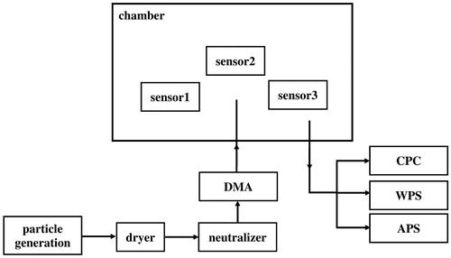
Figure 2. Size distribution of particles used for sensor calibration. (a) Ammonium sulfate; (b) sodium chloride.
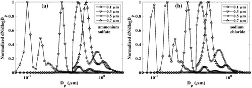
Figure 3. Time series of Plantower sensor number concentration signal at the channel >0.3 µm when 0.5 and 0.7 µm particles are tested: (a) ammonium sulfate; (b) sodium chloride.
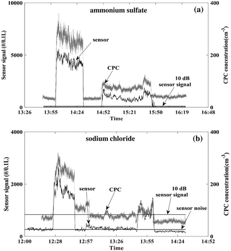
Figure 4. Calculated sensor transfer function at channel >0.3 µm using the method described in Section 2. The experimental data of ammonium sulfate particles of sizes 0.1, 0.3, 0.5, and 0.7 µm are used for the calculation.
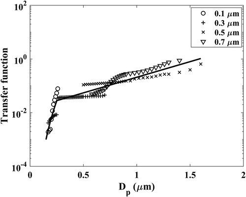
Figure 5. Light scattering curve with particle size. The markers are the corresponding values calculated from the Mie scattering theory, and the curves are the fitted ones.
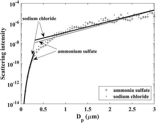
Figure 6. Sensor transfer function calculated from Tikhonov regularization (the markers) and the curve fitting (the lines) in the two size ranges (<0.3 µm and >0.3 µm) for the channel: (a) >0.3 µm; (b) >0.5 µm; (c) >1.0 µm; (d) >2.5 µm; (e) >5.0 µm; (f) >10 µm; (g) PM1; (h) PM2.5; (i) PM10.
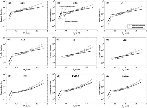
Table 1. Parameters for the sensor transfer function curve fit shown in .
Figure 7. Comparison between the measured sensor signal and the prediction from the transfer function developed in this study (a) particle number concentration for the six size channels; (b) three particle mass concentrations. The uncertainty in measured signal value is determined using error propagation of the maximum deviation from the average value of the three sensors during the entire experimental validation period. The uncertainty in predicted values is defined as the standard deviation of total particle number concentration measured by the CPC during the validation period.
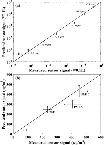
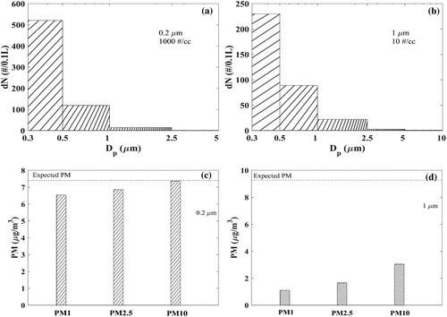
Figure 8. Predicted sensor signal for ammonium sulfate particles based on the transfer function fitting curves in . (a) Size distribution signal from 1000 cm−3 0.2 µm particles; (b) size distribution signal from 10 cm−3 1.0 µm particles; (c) PM signal from 1000 cm−3 0.2 µm particles; (d) PM signal from 10 cm−3 1.0 µm particles. The dashed lines at (c) and (d) are calculated mass concentrations based on spherical particle assumption.