Evaluation of low-cost optical particle counters for monitoring individual indoor aerosol sources

Figures & data

Figure 1. Schematic of the chamber experiment set-up.

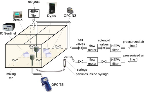
Table 1. Summary of the tested particle sensor characteristics.

Low-cost and reference sensors	Particle detection technology	Light source wavelength (nm)	Detection size range (µm)	# of bins	Bin size cuts (µm)	Flow rate (L/min)	Measurement time resolution (s)	Concentration detection limit
OPC N2 (Alphasense)	Laser diode	658^2	0.38–17	16	0.46, 0.66, 0.92, 1.20, 1.47, 1.83, 2.54, 3.50, 4.50, 5.75, 7.25, 9.00, 11.00, 13.00, 15.00, 16.75	Sampling: 0.22, total:1.2	1	3.40 × 10^11 particles/m^3
IC Sentinel	Laser diode, 10 mW	650^3	0.5-NR^6	4	0.5, 1, 5, 10	1.5	120	1.32 × 10^11 particles/m^3
Speck^1	LED	850^4	0.5–3	1	2	NR^6	30	NR^6
Dylos (DC1100)	NR^6	650	>1	2	1,5	0.283	60	NR^6
AeroTrak (TSI 9306)	Enhanced active cavity HeNe laser	785^5	0.3–14	6	0.3, 0.5, 1.0, 3.0, 5.0, 10.0	2.83	1	1.40 × 10^11 particles/m^3 at 5% coincidence loss

1: Uses DSM501A (Syhitech DSM501, Syhitech Co., Ltd) sensor.

2: Laser diode.

3: Laser diode, 10 mW.

4: LED.

5: Enhanced active cavity HeNe laser.

6: Not reported.

Figure 2. Particle size distribution of tested polydisperse particles during the first minute of particle injection measured by the reference sensor (AeroTrak, TSI): (a) dust mite, (b) pollen, (c) cat fur, (d) dog fur, and (e) quartz.

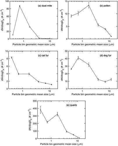
Table 2. Summary of the tested particles.

Particle type	Size distribution type	Size range (µm)	Biological/ non-Biological	Density (kg/m^3)	Shape	Roughness	Refractive index
Dust mite	Polydisperse	0.58–48^a	Biological	1140^a	Rounded**^,b	Smooth	–
Pollen	Polydisperse	–	Biological	850^b	Near spherical^b	–	1.5^c
Cat fur	Polydisperse	0.58–409^a	Biological	1000^a	Fibers^a	Rough	1.35–1.43^d
Dog fur	Polydisperse	0.58–35^a	Biological	1000^a	Fibers^a	Rough	1.37–1.55^d
Melamine resin (MF-R)	Monodisperse	1.041 ± 0.03*, 2.81 ± 0.06*	Non-biological	1510^e	Spherical^e	Smooth^e	1.68^e
Silicon dioxide (SiO2-R)	Monodisperse	0.977 ± 0.026*, 2.81 ± 0.1*	Non-biological	1850^e	Spherical^e	Smooth^e	1.5^f
Crushed quartz (>95% of SiO2)	Polydisperse	0.58–22.5^a	Non-biological	2650^a	Varied***^,a	Smooth	1.544^b

* Size ± standard deviation.

** With prismatic edges resulted from the ball mill crushing effect).

*** Varied from squares to rectangles (5/1 ratios maximum).

^aParticle size distribution is shown in Figure 2 and density information is based on a previous study (Salimifard et al. 2017).

^bHinds (2012).

^cGullvåg (1964).

^dYan et al. (2015).

^eAs provided by the manufacturer.

^fRadhakrishnan (1947).

Table 3. Tested sensors’ size bins representing particles smaller than 2.5 µm.

Low-cost and reference sensors	Size detection range (µm)
OPC N2 (Alphasense)	0.38–3
IC Sentinel	0.5–5
Speck	0.5–3
Dylos (DC1100)	1–5
AeroTrak (TSI 9306)	0.3–3

Figure 3. Time-series of dust mite particle number concentrations for the size range <2.5 µm measured by four low-cost sensors and the reference sensor. The test consists of three phases; 1) background level (minutes 0–5), 2) particle injection (minutes 5–7), and 3) particle concentration decay (minutes 7–150). Note that other test cases with different particle types and sizes had fairly similar temporal concentration profile trends.

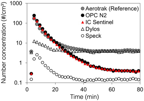
Figure 4. Particle number concentrations measured by low-cost sensors (y-axis) versus the reference sensor (x-axis). Subplots in the left column (a, c, e, and g) represent the non-linear response region (0–5/cm³). Subplots in the right column (b, d, f, and h) represent the linear response region.

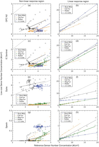
Table 4. Summary of regression analysis results for four tested bioaerosols comparing each low-cost sensor to the lab-grade sensor.

Particle type	Concentration range^a (#/cm^3)	OPC N2				IC Sentinel
		FB^b(#/cm^3)	PB^c	R^2	RMSE (#/cm^3)	FB (#/cm^3)	PB	R^2	RMSE (#/cm^3)
Dust mite	0–5	–2.64	0.751	0.320	0.250	–2.19	0.645	0.342	0.204
	5–20	–6.11	1.56	0.999	0.225	–5.39	1.37	0.999	0.194
Pollen	0–5	–1.17	0.556	0.248	0.350	–1.31	0.611	0.274	0.360
	5–20	–3.08	1.15	0.998	0.276	–3.30	1.20	0.998	0.255
Cat fur	0–5	–0.710	0.298	0.213	0.244	–0.740	0.330	0.213	0.272
	5–20	–2.77	0.875	0.997	0.146	–1.04	0.713	0.850	0.987
Dog fur	0–5	N/A				–1.53	0.508	0.645	0.131
	5–20					–4.53	1.15	0.997	0.278
Particle type		Speck				Dylos
	Concentration range^a (#/cm^3)	FB^b(#/cm^3)	PB^c	R^2	RMSE (#/cm^3)	FB (#/cm^3)	PB	R^2	RMSE (#/cm^3)
Dust mite	0–5	0.123	0.00343	0.00387	0.0125	3.55	0.0459	0.00163	0.259
	5–20	0.0158	0.0258	0.974	0.0214	3.24	0.128	0.918	0.192
Pollen	0–5	–0.0906	0.0310	0.161	0.0256	2.26	0.546	0.0645	0.752
	5–20	–0.404	0.0914	0.961	0.0915	2.71	0.467	0.977	0.360
Cat fur	0–5	–0.151	0.0454	0.176	0.0421	–0.242	0.0975	0.200	0.084
	5–20	–0.244	0.105	0.708	0.223	–1.89	0.418	0.957	0.291
Dog fur	0–5	–0.259	0.0718	0.402	0.0305	–0.443	0.180	0.523	0.0599
	5–20	–0.225	0.0613	0.983	0.0348	–1.39	0.369	0.998	0.0634

^aAs measured by the reference sensor.

^bFixed bias, intercept of regression model.

^cProportional bias, slope of regression model.

The results for each particle type are developed from one test.

Figure 5. The response of low-cost sensors under exposure to biological (a, c, e, and g) and non-biological (b, d, f, and h) aerosols with respect to the reference sensor.

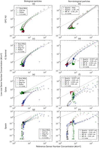
Figure 6. Regression analysis results of the low-cost sensors with respect to the reference sensor under exposure to common indoor bioaerosols. (a) Slope (proportional bias), (b) intercept (fixed bias), (c) R2 (linearity), and (d) RMSE (calibration precision). Please note that this plot does not include repetition tests. A similar plot that includes the regression results of the 2 repetition tests for dust mite particle is presented in Figure S3in the SI.

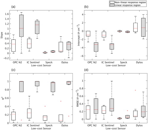
Table 5. Variation of the linear regression slopes of low-cost sensors response versus the reference sensor among different repetitions of three test particles.

Particle	Sensor	# of tests	Mean slope	S.E. of slope	Variation of slope
Dust Mite	IC Sentinel	3	1.16	0.0980	8.41%
	OPC N2	2	1.57	0.100	6.39%
	Speck	3	0.0468	0.0307	65.4%
	Dylos	3	0.182	0.112	61.5%
SiO2 – 2.81 µm	IC Sentinel	2	1.13	0.181	16.0%
	OPC N2	3	1.49	0.105	7.05%
	Speck	4	0.0285	0.00917	32.2%
	Dylos	3	0.253	0.0248	9.83%
MF-R – 2.81 µm	IC Sentinel	2	1.00	0.0982	9.82%
	OPC N2	2	1.30	0.0571	4.39%
	Speck	4	0.0398	0.0115	28.9%
	Dylos	4	0.290	0.0235	8.09%

Table 6. Linear calibration equations developed from tested bioaerosols (dust mite, pollen, cat fur, and dog fur) of smaller than 2.5 µm in concentrations of 5–20/cm³.

Low-cost sensor	Linear regression analysis results				Linear calibration equation
	FB(#/cm^3)	PB	R^2	RMSE (#/cm^3)
OPC N2	–4.92	1.32	0.920	1.66	${\mathrm{NC}}_{\mathrm{LCS},\mathrm{corrected}}=3.73+0.760 {\mathrm{NC}}_{\mathrm{LCS}}$
IC Sentinel	–4.55	1.22	0.953	1.15	${\mathrm{NC}}_{\mathrm{LCS},\mathrm{corrected}}=3.73+0.820 {\mathrm{NC}}_{\mathrm{LCS}}$
Speck	–0.176	0.0633	0.593	0.222	${\mathrm{NC}}_{\mathrm{LCS},\mathrm{corrected}}=2.78+15.8 {\mathrm{NC}}_{\mathrm{LCS}}$
Dylos	0.0210	0.405	0.373	2.22	${\mathrm{NC}}_{\mathrm{LCS},\mathrm{corrected}}=-0.0519+2.47 {\mathrm{NC}}_{\mathrm{LCS}}$

Salimifard, P., D. Rim, C. Gomes, P. Kremer, and J. D. Freihaut. 2017. Resuspension of biological particles from indoor surfaces: Effects of humidity and air swirl. Sci. Total Environ. 583 (April):241–7. doi:10.1016/j.scitotenv.2017.01.058.

 PubMed Web of Science ®Google Scholar

Hinds, W. C. 2012. Aerosol technology: Properties, behavior, and measurement of airborne particles. Wiley. ISBN: 978-0-471-19410-1.

 Google Scholar

Gullvåg, B. M. 1964. Morphological and quantitative investigations of pollen grains and spores by means of the Françon-Johansson interference microscope. Grana Palynol. 5 (1):3–23. doi:10.1080/00173136409429127.

 Google Scholar

Yan, L.-Q., C.-W. Tseng, H. W. Jensen, and R. Ramamoorthi. 2015. Physically-accurate fur reflectance. ACM Trans. Graph. 34 (6):1–13. doi:10.1145/2816795.2818080.

 Web of Science ®Google Scholar

Radhakrishnan, T. 1947. The dispersion, briefringence and optical activity of quartz. Proc. Indian Acad. Sci. 25 (3):260. doi:10.1007/BF03171408.

 Google Scholar