Multiparametric optical characterization of airborne dust with single particle extinction and scattering

Figures & data

Figure 1. Schematic of the optical layout. The 635 nm wavelength laser beam is expanded and focused into the flow cell, where particles are driven through its focal region. The air flow (∼dm³min⁻¹) is perpendicular to the beam, the air inlet is indicated with a circle in the figure. The emerging beam is collected in the forward direction by the QPD. Light power scattered toward the elliptical mirror in the lower part of the flow cell in this drawing is collected by the P90 sensor. The collection solid angle is 1.2 sr. The light scattered toward the P45 sensor is collected directly within a solid angle of about 0.01 rad.

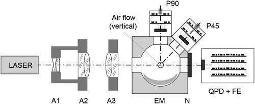
Figure 2. Examples of the raw data entering the asynchronous procedure to perform the offset follower. (a) Conditions of limited noise, with an average discrepancy 1: the trigger reset is active, and the trigger level is updated. (b) Noise conditions, with an average discrepancy 5: reset is prevented.

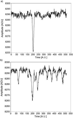
Figure 3. Examples of the results obtained with pure water droplets. Panel (a) represents ${(C}_{\mathit{ext}},\mathrm{ }\rho )$ pairs data as a 2 D histogram, where greytones indicate the relative number of events recorded within the 2 D bin. Panel (b) shows $(C_{\mathit{ext}},\mathrm{ }F(0)),$ $(C_{\mathit{ext}},F(45))$ and $(C_{\mathit{ext}},F(90))$ (from top to bottom), compared to the results of Mie calculations (solid lines). In (c) we report the results obtained for the values of the phase function obtained from (b), compared to the corresponding expected values (solid lines). (d) comparison of the phase functions obtained by fitting experimental data (solid line, black) and through Mie theory for the ensemble of droplets (circles, grey).

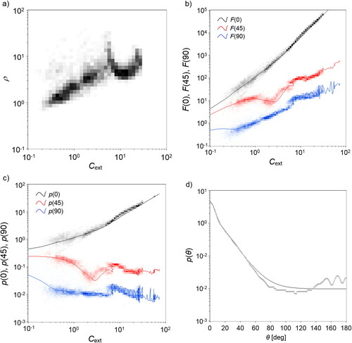
Figure 4. Results obtained in the city of Milan. Panels (a) (b) and (c) show data represented as in Figures 3a, b and c, respectively. Data on the right of the vertical line (C_ext>3) are multiplied by a factor of 10. Solid lines represent the Mie curves for water droplets for comparison. Notice the presence of two populations in (a). In (d) we show the phase functions fitted for the dielectric (solid line, black) and absorbing (circles, grey) portions of the population.

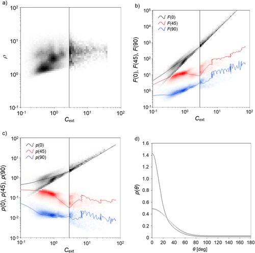
Table 1. Numerical results obtained with the established LibRadTran software package and the UVspec RTM as described in the text, to compare the influence of different sets of optical parameters obtained from the data in Figure 4. Mix: two populations; Die: purely dielectric; Inv: Mie inversion. Spectral irradiance values are expressed in mWm⁻²nm⁻¹.

	Mix	Die	Inv	Die-Mix	Inv-Mix
Edir	909	909	909	0	0
Edn	203	207	238	4	35
Eglo	1112	1116	1147	4	35
Eup	84.4	86	58	1.6	−26.4
Eabs	63.6	58	55	−5.6	−8.6