Interpretation of Volatility Tandem Differential Mobility Analyzer (V-TDMA) data for accurate vapor pressure and enthalpy measurement: Operational considerations, multiple charging, and introduction to a new analysis program (TAO)

Figures & data

Figure 1. The experimental apparatus used to test the charge separation hypothesis. The V-TDMA mode (blue dashed) confirms the presence of the bimodal volatility response. The extra classifier mode (red dotted) selects a portion of the bimodal response, re-neutralizes the classified particles, and uses DMA2 and the CPC to confirm the number of charges on the selected particles.

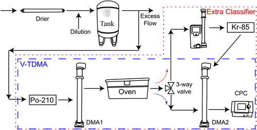
Figure 2. Measured CPC responses for the evaporation of levoglucosan are compared to model results, which represent the charge separation hypothesis. Panel (a) shows the CPC response from the V-TDMA mode, while panels (b) and (c) show the resulting CPC response when the extra classifier is included in the experimental set-up using set points of 47 nm and 78 nm, respectively. The peaks of the populations with different charges (post-Po-210 neutralizer → post-Kr-85 neutralizer) are indicated below the abscissa.

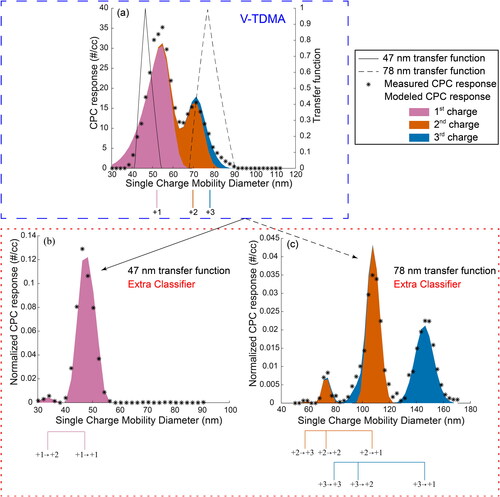
Figure 3. Panel (a): The modeled CPC response from the progressive evaporation of levoglucosan using an aerosol-to-sheath ratio of 1:10, a DMA1 set point of 90 nm, and the first size distribution (Sz Dist 1). Panel (b): The modeled CPC response using an aerosol-to-sheath ratio of 1:10, a DMA1 set point of 200 nm, and the first size distribution. Panel (c): The modeled CPC response using an aerosol-to-sheath ratio of 1:4, a DMA1 set point of 90 nm, and the first size distribution. Panel (d): The modeled CPC response using an aerosol-to-sheath ratio of 1:4, a DMA1 setpoint of 90 nm, and the second size distribution (Sz Dist 2).

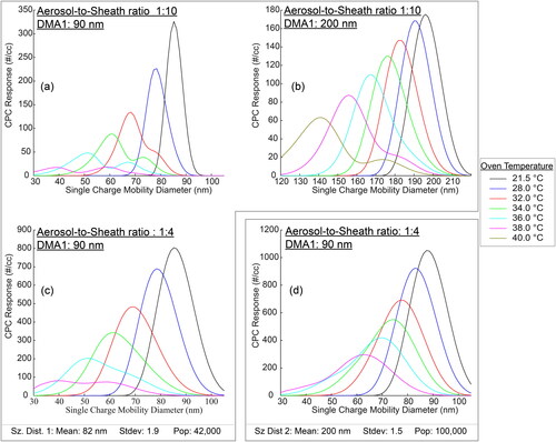
Figure 4. Modeled CPC responses for the evaporation of levoglucosan at 28 °C is shown for different size distributions (a) mean = 82 nm, standard deviation = 1.9, N = 42,000; (b) mean = 200 nm, standard deviation = 1.5, N = 100,000). In both cases, the aerosol-to-sheath flowrate ratio is 1:4, and the DMA1 setpoint is 90 nm. The peaks for the CPC response as well as the singly charged CPC response are indicated below the abscissa.

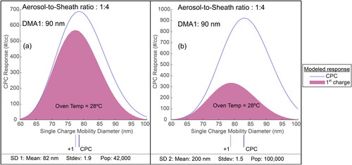
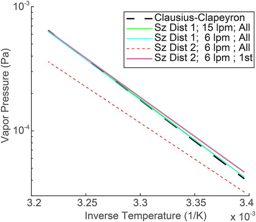
Figure 5. Clausius–Clapeyron plots from the different modeled situations. The dashed line is the actual Clausius–Clapeyron relationship assumed to develop all hypothetical situations. The multi-charged situation (size distribution 2) in combination with the wide transfer function (sheath flow rate of 6 lpm) creates errors in both vapor pressure and enthalpy measurements (red dotted). If the actual location of the singly charged particles is known, (for example, if instrument settings are used to force the separation of the singly charged particles from the multiply charged particles) then the correct relationship is recovered (thick purple).