Toward elemental analysis of ambient single particles using electrodynamic balance and laser-induced breakdown spectroscopy

Figures & data

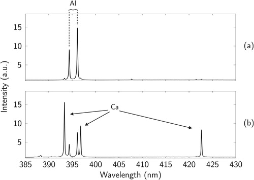
Figure 1. A schematic cross-section of the developed charger and a simulation of the electric field strength around the inner tube. Dimensions of the inner and outer tubes are 2.0 mm and 13 mm (ID), respectively. Aerosol flows through the inner tube through the corona discharge, leading to an electric field of the order 10⁵–10⁶ Vm⁻¹ in the charging region.

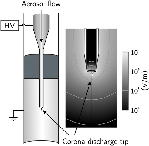
Figure 2. The characterization setups of the charger and the EDB. SCAR provides singly charged aerosol, which is classified into a monodisperse aerosol with the tampere long DMA. The monodisperse aerosol is then charged and directed into one of the three alternative measurement branches, which are used one at a time.

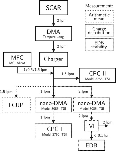
Figure 3. Calculated stability areas of a particle in an EDB using the dimensionless stability parameters presented in Equation (6)(6) $$\frac{{\mathrm{d}}^{2}Z}{\mathrm{d}\tau }+\delta \frac{\mathrm{d}Z}{\mathrm{d}\tau }+2\beta Z\text{cos}\left(2\tau \right)=\sigma ,$$(6) . Particles with charging states achieved with the charger presented in the previous chapter should be well in the stable area of the chart with an amplitude AC-voltage of 1 kV and an AC-frequency of 100 Hz.

Figure 4. A schematic figure of the EDB-LIBS measurement principle (a) and of the used optical chamber (b). An aerosol enters the charger with a 2 lpm flow rate, which is also the major flow of the virtual impactor. The minor flow of the virtual impactor continues to the EDB chamber with a flow rate below 0.1 lpm.

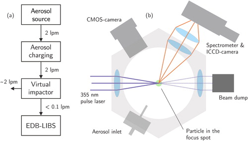
Figure 5. An example charge distribution measurement at the particle size of 0.760 µm, including the mean values and a log-normal fit to the measurement points.

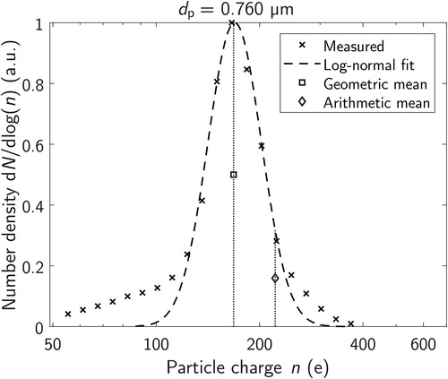
Figure 6. A comparison between the characterized charger, theoretical equations and selected previously presented aerosol chargers. Literature results are the arithmetic mean values of the chargers under consideration.

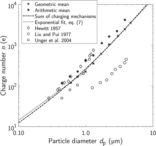
Figure 7. Measured threshold voltages with different electrical mobilities, sizes and initial positions as a function of the calculated threshold value from Equation (8)(8) $$V_{\mathrm{AC}}^{\mathrm{*}}=\frac{z_0}{Z{C}_1}\sqrt{\frac{3g{z}_{\mathrm{i}}{C}_2}{2C_0}},$$(8) .

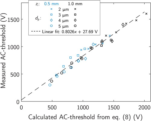
Figure 8. Threshold charge numbers required for successful balancing of a particle as a function of particle size with different (1, 2, and 4 kV) amplitude AC-voltages. The figure includes the measured geometric and arithmetic mean values and the Rayleigh limit charge, which is considered as the maximum charge for liquid particles. The 4 kV value was experimentally estimated to be the maximum safe operating amplitude.

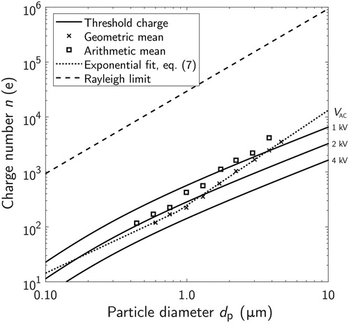
Figure 9. The spectra from the laboratory study of dry generated (a) and wet generated (b) kaolinite particles. Both spectra consists of ca. 10 averaged particle hits and are divided with the background signal from ambient air.