Diffusional transfer function for the scanning electrical mobility spectrometer (SEMS)

Figures & data

Figure 1. Schematic representation of the flows and particle trajectories in the cross section of a simplified DMA by ignoring the transition flows at the inlet and outlet of the column DMA, which is a cylindrical annulus. R₁ and R₂ are the inner and outer radii of the annulus, L is the length of DMA, $Q_{\text{sh}},Q_{\mathrm{a}},Q_{\text{ex}},$ and $Q_{\mathrm{c}}$ are the sheath (gray arrow), aerosol (orange arrow), excess (green arrow), and classified (red arrow) flows. The boundaries of the regimes of each flow are marked by dashed lines. Laminar flow is assumed (magenta curve). The outer wall of the DMA is grounded and the inner wall is applied with high negative voltage; thus a radial (from outer to inner) electrical field drives positively charged particles migrating from the outer to inner wall while moving downstream with the flow. The curves (in blue, green, and red) are particle trajectories corresponding to three scenarios that particles end in the excess flow regime, the classified flow regime, and the wall. Only trajectories ending in the classified flow regime are counted in deriving the DMA transfer function.

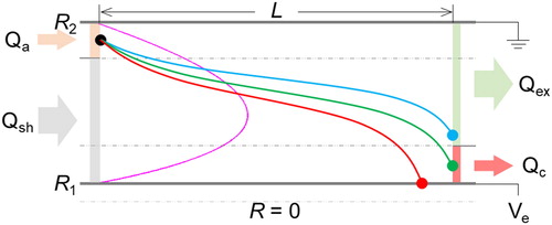
Figure 2. Trajectories of non-diffusive particles of the same mobility in a scanning DMA ($\beta =\frac{1}{10},$ δ = 0, and ${\tau }_s=1$). Starting from ${\tau }_t=0,$ particles of the same mobility are continuously injected into the scanning DMA at the inlet. Only those that enter the DMA at a specific entering time and position can successfully transmit through the DMA. The reference trajectory (yellow curve) has an entering time ${\tau }_i=0$ and an entering position ${\omega }_i=1,$ ending at ${\omega }_e={\omega }_c$ with a transit time ${\tau }_t=1.13.$ For those that start at ${\omega }_i=1$ and end at ${\omega }_e=\gamma$ (red curve), the entering time must be later than 0 and the corresponding transit time is somewhat longer than the reference. For particles starting at ${\omega }_i={\omega }_a$ and ending at ${\omega }_e={\omega }_c$ (purple curve), the transit time is the shortest among all the trajectories but particles enter the DMA at a much later time. For those that start at ${\omega }_i={\omega }_a$ and end at ${\omega }_e=\gamma$ (blue curve), particles have to enter the scanning DMA at the latest time but with a relatively short transit time. The order of the exiting time (${\tau }_i+{\tau }_t,$ purple < yellow < blue < red) of the four trajectories is not the same as the entrance time (τ_i), indicating the complexity of the motion of particles in a scanning DMA.

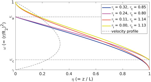
Figure 3. Contour plots of relative electrical mobility that can transmit through the static DMA ($\beta =\frac{1}{10},$ and δ = 0), ${}^s\zeta ,$ in the (a) position (ω_i, ω_e) and (b) flow fraction (F_i, F_e) coordinates. Each point in the contour plot represents the particle trajectory that starts from the location ω_i or the flow fraction F_i at the inlet and ends at the location ω_e or the flow fraction F_e at the outlet. The color of contour lines corresponds to different values of the relative electrical mobility ${}^s\zeta ,$ which is calculated from Equation (16)(16) $${}^s\zeta =(1+\beta )A_{\gamma }\{{\omega }_i\left(\hspace{0.17em}\text{ln}\hspace{0.17em}{\omega }_i-1\right)-{\omega }_e\left(\hspace{0.17em}\text{ln}\hspace{0.17em}{\omega }_e-1\right)-\frac{{\omega }_i-{\omega }_e}{1-\gamma }\left(1-\frac{{\omega }_i+{\omega }_e}{2}\right)\hspace{0.17em}\text{ln}\hspace{0.17em}\gamma \}$$(16) as a function of ω_i and ω_e, and the transformation from space ω to flow fraction $F(\omega )$ is realized by Equation (17)(17) $$F(\omega )={(1-\gamma )}^{-1}{\int }_{\omega }^1\tilde{u}(\omega \prime )d\omega \prime =-A_{\gamma }\left[\omega \hspace{0.17em}\text{ln}\hspace{0.17em}\omega -\omega +1+\frac{{(1-\omega )}^2}{2(1-\gamma )}\text{ln}\hspace{0.17em}\gamma \right]$$(17) . The contour lines in the position coordinate are curved, while those in the flow fraction coordinate are equally spaced straight lines, which adhere to Equation (18)(18) $${}^s\zeta =(1+\beta )\left(F_e-F_i\right)$$(18) .

Figure 4. Contour plot of relative electrical mobility in the scanning DMA ($\beta =\frac{1}{10},$ δ = 0, and ${\tau }_s=1$) within the flow fraction coordinate. The relative electrical mobility in the scanning DMA is calculated by Equations (10), (15)(15) $$\frac{1}{{\tau }_s{A}_{\gamma }}=(1-\gamma )\left[{\theta }_t\hspace{0.17em}\text{ln}\hspace{0.17em}({\omega }_e+\lambda )-{\text{Li}}_2\left(\frac{\lambda }{{\omega }_e+\lambda }\right)+{\text{Li}}_2\left(\frac{\lambda }{{\omega }_e+\lambda }{\mathrm{e}}^{-{\theta }_t}\right)\right]-\hspace{0.17em}\text{ln}\hspace{0.17em}\gamma \left[{\theta }_t(1-{\omega }_e-\lambda )+{\omega }_i-{\omega }_e\right]$$(15) , and (17)(17) $$F(\omega )={(1-\gamma )}^{-1}{\int }_{\omega }^1\tilde{u}(\omega \prime )d\omega \prime =-A_{\gamma }\left[\omega \hspace{0.17em}\text{ln}\hspace{0.17em}\omega -\omega +1+\frac{{(1-\omega )}^2}{2(1-\gamma )}\text{ln}\hspace{0.17em}\gamma \right]$$(17) . Each point in the contour plot represents the particle trajectory that starts from the flow fraction F_i at the inlet and ends at the flow fraction F_e at the outlet. The contour lines are curved compared with the straight lines in the static DMA F_i-F_e plot (Figure 3), indicating the effect of scanning on the distribution of the transmission of particles of different electrical mobility.

Figure 5. Contour plots of the residence time τ_t distribution in (a) static and (b) up-scanning modes ($\beta =\frac{1}{10},$ δ = 0, and τ_s = 1). The residence time for the static DMA is calculated from Equations (12)(12) $${}^s{\theta }_t=\frac{{\omega }_i-{\omega }_e}{{}^s\lambda }$$(12) and (16)(16) $${}^s\zeta =(1+\beta )A_{\gamma }\{{\omega }_i\left(\hspace{0.17em}\text{ln}\hspace{0.17em}{\omega }_i-1\right)-{\omega }_e\left(\hspace{0.17em}\text{ln}\hspace{0.17em}{\omega }_e-1\right)-\frac{{\omega }_i-{\omega }_e}{1-\gamma }\left(1-\frac{{\omega }_i+{\omega }_e}{2}\right)\hspace{0.17em}\text{ln}\hspace{0.17em}\gamma \}$$(16) , while those for the scanning DMA is calculated from Equations (10)(10) $${\theta }_t=\hspace{0.17em}\text{ln}\hspace{0.17em}\left(\frac{\lambda }{\lambda -{\omega }_i+{\omega }_e}\right)$$(10) and (15)(15) $$\frac{1}{{\tau }_s{A}_{\gamma }}=(1-\gamma )\left[{\theta }_t\hspace{0.17em}\text{ln}\hspace{0.17em}({\omega }_e+\lambda )-{\text{Li}}_2\left(\frac{\lambda }{{\omega }_e+\lambda }\right)+{\text{Li}}_2\left(\frac{\lambda }{{\omega }_e+\lambda }{\mathrm{e}}^{-{\theta }_t}\right)\right]-\hspace{0.17em}\text{ln}\hspace{0.17em}\gamma \left[{\theta }_t(1-{\omega }_e-\lambda )+{\omega }_i-{\omega }_e\right]$$(15) . Note the different ranges of the color bar. Particles experience longer time in the DMA when the voltage is scanning.

Figure 6. Non-diffusive transfer functions of the static DMA ($\beta =\frac{1}{10}$) translated from contour plots of relative mobility distribution in inlet-exit flow fraction coordinate for (a) balanced inlet and exit flows (Q_a = Q_c, i.e., δ = 0 as defined in Equation (6)(6) $$\delta =\frac{Q_{\mathrm{c}}-Q_{\mathrm{a}}}{Q_{\mathrm{c}}+Q_{\mathrm{a}}}$$(6) ), (b) higher inlet flow ($Q_a=2Q_c,$ i.e., $\delta =-1/3$), and (c) higher exit flow ($Q_a=\frac{1}{2}{Q}_c,$ i.e., $\delta =1/5$). The contour plots on the left column are calculated from Equation (18)(18) $${}^s\zeta =(1+\beta )\left(F_e-F_i\right)$$(18) , and the dots in the plots on the right column are the transfer function calculated from Equation (19)(19) $$\Omega (Z;Z^{†}(t_e))={\int }_0^{\frac{\beta (1-\delta )}{1+\beta }}\left[{\int }_{1-\frac{\beta (1+\delta )}{1+\beta }}^1{f}_{\text{trans}}(F_e;F_i)d{F}_e\right]f_{\text{inlet}}(F_i)d{F}_i$$(19) , while the lines are the transfer function calculated from Equation (S15). The shades (light blue) on the contour plots indicate the range of the contour lines that correspond to the highest values of the transfer function.

Figure 7. Non-diffusive transfer functions of static and up-scanning modes (with different ramping time, where $\beta =\frac{1}{10},$ δ = 0, and ${\tau }_s=$ 5, 2, and 1, respectively). The scanning DMA transfer function shifts peak position to larger values and widens peak width compared with the static case. The Stolzenburg transfer function (dots) is calculated from Equation (S15).

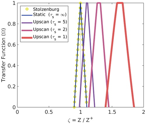
Figure 8. Diffusive trajectories in the DMA. The flow boundaries, flow rates, and particle trajectories are the same as those in Figure 1. Assuming the diffusion process adheres to the Gaussian distribution, the end of the trajectory has a probability distribution, only those of which lie within the outflow regime (Q_c, shaded area) are counted in calculating the transfer function. For particles that end out of Q_c (the blue trajectory), after considering diffusion, those particles still have some probability to penetrate the DMA (the right tail of the Gaussian distribution); while for those that end at the inner wall of the DMA (the red trajectory), the left tail of the Gaussian distribution lies within Q_c; thus some number fraction of these particles can still successfully transmit through the DMA.

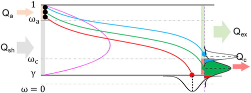
Figure 9. Extended flow fraction regime in the diffusional case. The solid square (yellow) represents the original F_i-F_e space, while the dashed square (yellow) identifies the boundary of the extended F_i-F_e space. The dots (blue, green, and red) correspond to the three trajectories in Figure 8, and the shaded area inside the solid square regime represents the probability of a particle penetrating the DMA.

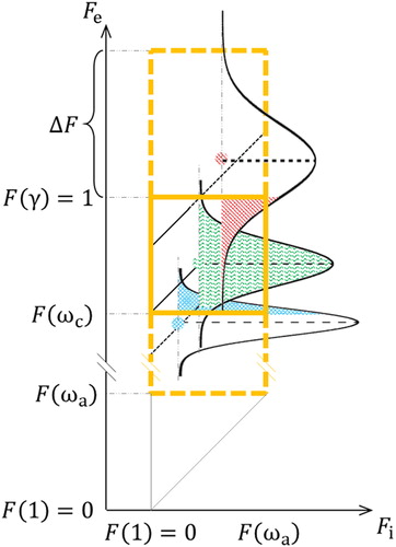
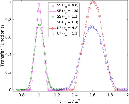
Figure 10. Diffusional DMA transfer functions in static (left curves) and up-scan (right curves) mode for the exit voltage at ${\tau }_e=1.3$ and 4.8 ($\beta =\frac{1}{10},$ δ = 0, ${\tau }_s=1,Q_{\text{sh}}=2.5$ LPM, $V_{\text{min}}=15$ V, $V_{\text{max}}=9850$ V, and TSI 3081 column DMA), respectively. “SS” stands for static mode with Stolzenburg equation (Equation (S16)), “SF” stands for static mode with flow fraction contour integral, and “UF” stands for up-scanning mode with flow fraction contour integral. For static mode, the diffusional DMA transfer functions calculated from Equation (S16) and the integral over flow fraction contour lines overlap very well. For up-scan mode, when particle diffusion is considered, the transfer function is no longer trapezoid. As τ_e gets smaller, the height of the peak is $\sim 0.75$ and the width of the peak becomes broader (in this example, ${\tau }_e=1.3$ corresponds the diameter of 41 nm and ${\tau }_e=4.8$ corresponds to 812 nm). Thus particle diffusion extends the range of particle mobilities that can transmit through the scanning DMA, smooths the shape of the peak and lowers the height of the scanning transfer function.