
Figures & data
Figure 1. Frequency distribution of for one example population (
) and different sample sizes. For each sample size, the sampling process was repeated 1000 times. The dashed colored lines correspond to the average
for the specified sample size.
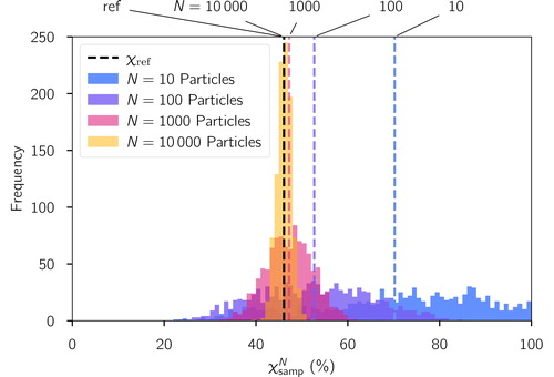
Figure 2. Distribution of sampled population mixing-state index and reference mixing-state index χref for increasing sample sizes based on the simulated scenario library described in Section 2.3. The solid black line is the 1:1 line.
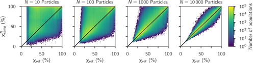
Figure 3. Sampled as a function of χref from data obtained in Pittsburgh, PA. The one-to-one line is drawn for reference.
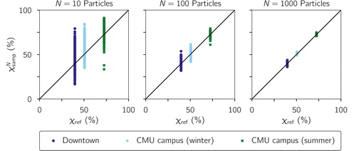
Figure 4. Distribution of average sampled (averaged over the 1000 repeats) and χref for increasing sample sizes based on the simulated scenario library described in Section 2.3. The one-to-one line is drawn for reference.
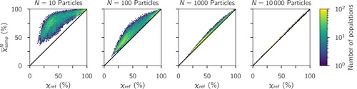
Figure 5. Distribution of average sampled (mean particle diversity, averaged over the 1000 repeats) and
(reference mean particle diversity) for increasing sample sizes based on the simulated scenario library described in Section 2.3. The one-to-one line is drawn for reference.
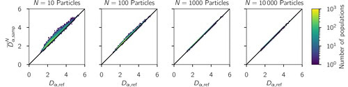
Figure 6. Distribution of average sampled (total diversity, averaged over the 1000 repeats) and
(reference total diversity) for increasing sample sizes based on the simulated scenario library described in Section 2.3. The one-to-one line is drawn for reference.
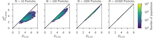
Figure 7. 95%-Confidence intervals for sampled values for sample sizes of N = 10, 100, 1000, and 10,000 particles based on the simulated scenario library described in Section 2.3.
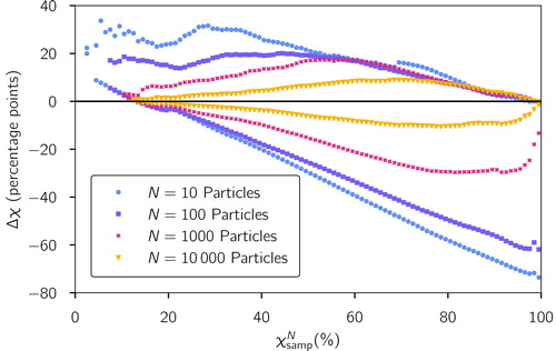
Figure 8. Schematic to illustrate Theorem 3. Here we consider two sampled populations with α-diversities of and
which we assume have average exactly equal to the reference value
(this is true on average, as we saw from Theorem 1). The exponential function maps entropies H to diversities D, and because it is convex the average sampled value,
will be greater than the reference value,
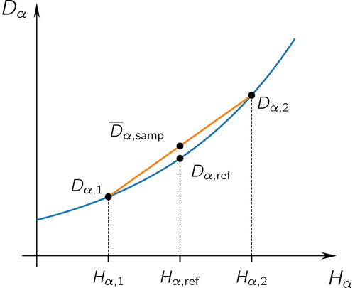
Figure 9. Schematic to illustrate Theorem 4 in the case of a two-species aerosol population, where p is the mass fraction of the first species. We consider two sampled populations with first-species mass-fractions of p1 and p2, which we assume have average exactly equal to the first-species reference mass fraction of pref (this is exactly true on average by (Equation43(43)
(43) )). The diversity function is concave (for 2 or 3 species) so the average sampled value,
will be less than the reference value,
![Figure 9. Schematic to illustrate Theorem 4 in the case of a two-species aerosol population, where p is the mass fraction of the first species. We consider two sampled populations with first-species mass-fractions of p1 and p2, which we assume have average exactly equal to the first-species reference mass fraction of pref (this is exactly true on average by (Equation43(43) Es∼ps,tot[Ei∼ps,i[Xs,i]︸Xs,tot]=EI∼pI[XI].(43) )). The diversity function is concave (for 2 or 3 species) so the average sampled value, D¯γ,samp, will be less than the reference value, Dγ,ref.](/cms/asset/32bdba83-f365-4a98-bb3d-2b8e590a493c/uast_a_1804523_f0009_c.jpg)
Data availability
The output of the particle-resolved modeling scenario library can be accessed at https://doi.org/10.13012/B2IDB-2774261_V1.