Accelerated measurements of aerosol size distributions by continuously scanning the aerodynamic aerosol classifier

Figures & data

Figure 1. Example of the transfer function (${\Omega }_{\text{AAC}}$) of the steady-state (ss) or scanning (sc) AAC based on limited trajectory theory (as summarized in Table 1), where ${\Omega }_{\text{AAC},\text{sc}}$ is shown at 15 different times (in terms of $t_{\text{in}}$ or $t_{\mathrm{m}}$) over a 600 s scan from ${\omega }_{\mathrm{S}}=20$ rad/s to ${\omega }_{\mathrm{E}}=700$ rad/s, while ${\Omega }_{\text{AAC},\text{ss}}$ is only shown at the start and end speeds of the scan (i.e., ${\omega }_{\mathrm{S}}$ and ${\omega }_{\mathrm{E}},$ respectively).

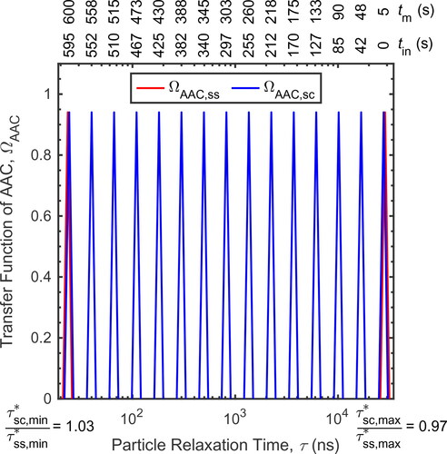
Figure 2. Example comparing the transfer function of the scanning AAC with balanced classifier flows based on limited trajectory or particle streamline theory.

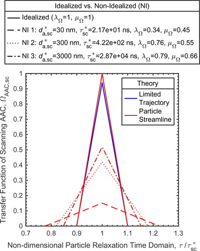
Figure 3. The average scanning AAC transfer function ${\Omega }_{\text{AAC}}$ based on idealized limited trajectory or non-idealized particle streamline theory over three different particle detector counting times ($t_{\mathrm{c}}$), where subplots (a), (b), and (c) show the transfer functions at the start of the up scan, end of the up scan and start of the down scan, respectively. The vertical line in each subplot, denoted with a black, dash-dot line style, shows the instantaneous setpoint of the scanning AAC (in terms of relaxation time, ${\tau }_{\text{sc}}^{\ast }$ or aerodynamic diameter³, $d_{\mathrm{a},\text{sc}}^{\ast }$) at the start of the counting interval of the particle detector.

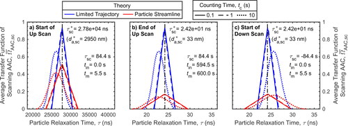
Table 1. Transfer function of the steady-state (ss) or scanning (sc) AAC based on limited trajectory (LT) theory.

Parameter	Equation	SI Eq. #
${\tau }_{\text{max}}$	$\frac{1}{K}\text{ln}\hspace{0.17em}\left(\frac{r_2}{r_1}\right)$ (20)	S3.5
${\tau }_{\text{min}}$	$\frac{1}{2K}\text{ln}\hspace{0.17em}(\frac{Q_{\mathrm{a}}+Q_{\text{sh}}-Q_{\mathrm{s}}(1-r_1^2/r_2^2)}{Q_{\mathrm{a}}+Q_{\text{sh}}-Q_{\text{sh}}(1-r_1^2/r_2^2)})$ (21)	S3.8
${\tau }^{\ast }$	$\frac{{\tau }_{\min }+{\tau }_{\max }}{2}$ (22)	S3.9
f1	$\frac{Q_{\mathrm{a}}+Q_{\text{sh}}{r}_1^2/r_2^2-\hspace{0.17em}\text{exp}\hspace{0.17em}(-2\tau K)\left[Q_{\mathrm{a}}+Q_{\text{sh}}-Q_{\mathrm{s}}(1-r_1^2/r_2^2)\right]}{Q_{\mathrm{a}}(1-r_1^2/r_2^2)}$ (23)	S3.12
f2	$\frac{Q_{\mathrm{a}}+Q_{\text{sh}}}{Q_{\mathrm{a}}}(\frac{\hspace{0.17em}\text{exp}\hspace{0.17em}(-2\tau K)-r_1^2/r_2^2}{1-r_1^2/r_2^2})$ (24)	S3.15
f3	$\frac{Q_{\mathrm{s}}}{Q_{\mathrm{a}}}$ (25)	S3.16
${\Omega }_{\text{AAC}}$	$\max [0,\min (f_1,f_2,f_3,1)]$ (26)	S3.17

Where K equals $K_{\text{ss}}$ (Equation (16)(16) $$\begin{array}{c}{K}_{\text{ss}}={\int }_{t_{\text{in}}}^{t_{\text{in}}+t_{\mathrm{f}}}{\omega }^2\mathrm{d}t\prime ={\omega }^2{t}_{\mathrm{f}},\hfill \end{array}$$(16) ) or $K_{\text{sc}}$ (Equation (19)(19) $$\begin{array}{c}{K}_{\text{sc}}(t_{\mathrm{m}})={\int }_{t_{\mathrm{m}}-t_{\mathrm{f}}}^{t_{\mathrm{m}}}{\omega }_{\mathrm{S}}^2\hspace{0.17em}\text{exp}\hspace{0.17em}\left(\frac{t}{{\tau }_{\text{sc}}}\right)\mathrm{d}t\prime \hfill \\ K_{\text{sc}}(t_{\mathrm{m}})={\omega }_{\mathrm{S}}^2{\tau }_{\text{sc}}\hspace{0.17em}\text{exp}\hspace{0.17em}\left(\frac{t_{\mathrm{m}}}{{\tau }_{\text{sc}}}\right)\left[1-\hspace{0.17em}\text{exp}\hspace{0.17em}\left(\frac{-t_{\mathrm{f}}}{{\tau }_{\text{sc}}}\right)\right].\hfill \end{array}$$(19) ) for the steady-state or scanning AAC, respectively.

Table 2. Transfer function of the scanning AAC based on particle streamline (PS) theory with balanced classifier flows or limited trajectory (LT) theory.

		Particle streamline (PS) with	SI Eq. #
Parameter	Limited trajectory (LT)	balanced (B) classifier flows	LT	PS
${\Omega }_{\text{AAC},\text{sc}}$	max[0, min(f1, f2, f3, 1)](27)	$\frac{{\lambda }_{\Omega }{\mu }_{\Omega }^2}{2\beta }[\left|\frac{\tau }{{\tau }_{\text{sc},\mathrm{B}}^{\ast }}-\left(1+\frac{\beta }{{\mu }_{\Omega }}\right)\right|+\left|\frac{\tau }{{\tau }_{\text{sc},\mathrm{B}}^{\ast }}-\left(1-\frac{\beta }{{\mu }_{\Omega }}\right)\right|-2\left|\frac{\tau }{{\tau }_{\text{sc},\mathrm{B}}^{\ast }}-1\right|]$ (28)	S3.17	S4.1
${\tau }_{\text{sc}}^{\ast }$	$c_{\tau \ast }\hspace{0.17em}\text{exp}\hspace{0.17em}\left(\frac{-t_{\mathrm{m}}}{{\tau }_{\text{sc}}}\right)$  (29)		S3.34	S4.10
$c_{\tau \ast }$	$\frac{1}{2c_{\text{sc}}}[\text{ln}\hspace{0.17em}\left(\frac{r_2}{r_1}\right)+\frac{1}{2}\text{ln}\hspace{0.17em}(\frac{Q_{\mathrm{a}}+Q_{\text{sh}}-Q_{\mathrm{s}}(1-r_1^2/r_2^2)}{Q_{\mathrm{a}}+Q_{\text{sh}}-Q_{\text{sh}}(1-r_1^2/r_2^2)})]$ (30)	$\frac{1}{c_{\text{sc}}}\frac{2(r_2^2-r_1^2)}{(\beta +1){(r_1+r_2)}^2}$ (31)	S3.36	S4.11
$c_{\text{sc}}$	${\omega }_{\mathrm{S}}^2{\tau }_{\text{sc}}\left[1-\hspace{0.17em}\text{exp}\hspace{0.17em}\left(\frac{-t_{\mathrm{f}}}{{\tau }_{\text{sc}}}\right)\right]$ (32)		S3.29	S4.12

Figure 4. A comparison of the non-dimensional deconvolution parameter (${\beta }_{\text{sc}}^{\ast }$) of the transfer function of the scanning AAC, where subplot (a) compares the parameters based on idealized limited trajectory or particle streamline theory, while subplots (b) and (c) compare the idealized and non-idealized³ deconvolution parameters based on particle streamline theory at two sample flows ($Q_{\mathrm{a}}=0.3$ or 1.5 L/min).

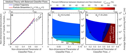
Table 3. Average transfer function of scanning AAC over counting time of the particle detector.

Parameter	Limited trajectory (LT)	Particle streamline (PS) with balanced (B) classifier flows	SI Eq. #
			LS	PS
${\overline{\Omega }}_{\text{AAC},\text{sc}}$	$$\begin{array}{l}\begin{array}{l}\left[\frac{c_{f11}{\tau }_{\text{sc}}}{t_{\text{c}}}\mathcal{E}\mathcal{I}\left(c_{\tau \min }{c}_{f12}\right)-\frac{c_{f13}}{t_{\text{c}}}\left(t_{\text{m}}-{\tau }_{\text{sc}}\ln \left(\frac{c_{\tau \min }}{\tau }\right)\right)\right]\left[\mathcal{H}\left(\tau -{\tau }_{\min }\right)-\mathcal{H}\left(\tau -{\tau }_{\min ,\text{tc}}\right)\right]\hfill \\ +\left[-\frac{c_{f11}{\tau }_{\text{sc}}}{t_{\text{c}}}\mathcal{E}\mathcal{I}\left(c_{f12}\tau \exp \left(\frac{t_{\text{m}}}{{\tau }_{\text{sc}}}\right)\right)\right]\left[\mathcal{H}\left(\tau -{\tau }_{\min }\right)-\mathcal{H}\left(\tau -{\tau }_{13}\right)\right]\hfill \\ \begin{array}{l}+\left[\frac{c_{f11}{\tau }_{\text{sc}}}{t_{\text{c}}}\mathcal{E}\mathcal{I}\left(c_{f12}\tau \exp \left(\frac{t_{\text{m}}+t_{\text{c}}}{{\tau }_{\text{sc}}}\right)\right)+c_{f13}\right]\\ \left[\mathcal{H}\left(\tau -{\tau }_{\min ,\text{tc}}\right)-\mathcal{H}\left(\tau -{\tau }_{13,\text{tc}}\right)\right]\end{array}\hfill \end{array}\\ \begin{array}{l}+\left[-\frac{c_{f11}{\tau }_{\text{sc}}}{t_{\text{c}}}\mathcal{E}\mathcal{I}\left(c_{\tau 13}{c}_{f12}\right)+\left(\frac{c_{f13}}{t_{\text{c}}}-\frac{c_{f31}}{t_{\text{c}}}\right)\left(t_{\text{m}}-{\tau }_{\text{sc}}\ln \left(\frac{c_{\tau 13}}{\tau }\right)\right)\right]\hfill \\ \left[\mathcal{H}\left(\tau -{\tau }_{13}\right)-\mathcal{H}\left(\tau -{\tau }_{13,\text{tc}}\right)\right]\hfill \\ +c_{f31}\left[\mathcal{H}\left(\tau -{\tau }_{13,\text{tc}}\right)-\mathcal{H}\left(\tau -{\tau }_{23,\text{tc}}\right)\right]\hfill \\ +\left[\frac{c_{f21}{\tau }_{\text{sc}}}{t_{\text{c}}}\mathcal{E}\mathcal{I}\left(c_{\tau 23}{c}_{f22}\right)+\left(\frac{c_{f31}}{t_{\text{c}}}-\frac{c_{f23}}{t_{\text{c}}}\right)\left(t_{\text{m}}-{\tau }_{\text{sc}}\ln \left(\frac{c_{\tau 23}}{\tau }\right)\right)\right]\hfill \\ \left[\mathcal{H}\left(\tau -{\tau }_{23}\right)-\mathcal{H}\left(\tau -{\tau }_{23,\text{tc}}\right)\right]\hfill \end{array}\\ \begin{array}{l}+\left[\frac{c_{f21}{\tau }_{\text{sc}}}{t_{\text{c}}}\mathcal{E}\mathcal{I}\left(c_{f22}\tau \exp \left(\frac{t_{\text{m}}+t_{\text{c}}}{{\tau }_{\text{sc}}}\right)\right)+c_{f23}\right]\hfill \\ \left[\mathcal{H}\left(\tau -{\tau }_{23,\text{tc}}\right)-\mathcal{H}\left(\tau -{\tau }_{\max ,\text{tc}}\right)\right]\hfill \\ +\left[-\frac{c_{f21}{\tau }_{\text{sc}}}{t_{\text{c}}}\mathcal{E}\mathcal{I}\left(c_{f22}\tau \exp \left(\frac{t_{\text{m}}}{{\tau }_{\text{sc}}}\right)\right)\right]\left[\mathcal{H}\left(\tau -{\tau }_{23}\right)-\mathcal{H}\left(\tau -{\tau }_{\max }\right)\right]\hfill \\ +\left[-\frac{c_{f21}{\tau }_{\text{sc}}}{t_{\text{c}}}\mathcal{E}\mathcal{I}\left(c_{\tau \max }{c}_{f22}\right)+\frac{c_{f23}}{t_{\text{c}}}\left(t_{\text{m}}-{\tau }_{\text{sc}}\ln \left(\frac{c_{\tau \max }}{\tau }\right)\right)\right]\hfill \\ \left[\mathcal{H}\left(\tau -{\tau }_{\max }\right)-\mathcal{H}\left(\tau -{\tau }_{\max ,\text{tc}}\right)\right]\hfill \end{array}\end{array}$$(42)	$$\begin{array}{l}\begin{array}{l}\left[-\frac{{\lambda }_{\Omega }{\mu }_{\Omega }{c}_{\text{BL}}}{t_{\text{c}}}\left(t_{\text{m}}-{\tau }_{\text{sc}}\ln \left(\frac{c_{\tau \min ,\text{B}}}{\tau }\right)\right)+\frac{c_{\text{B}2}{c}_{\tau \min ,\text{B}}}{c_{\tau \ast ,\text{B}}}\right]\hfill \\ \left[\mathcal{H}\left(\tau -{\tau }_{\min ,\text{B}}\right)-\mathcal{H}\left(\tau -{\tau }_{\min ,\text{B},\text{tc}}\right)\right]\hfill \\ +\left[-\frac{c_{\text{B}2}}{c_{\tau \ast ,\text{B}}}\tau \exp \left(\frac{t_{\text{m}}}{{\tau }_{\text{sc}}}\right)\right]\hfill \\ \left[\mathcal{H}\left(\tau -{\tau }_{\min ,\text{B}}\right)-\mathcal{H}\left(\tau -{\tau }_{\text{sc},\text{B}}^{\ast }\right)\right]\hfill \end{array}\\ \begin{array}{l}+\left[{\lambda }_{\Omega }{\mu }_{\Omega }{c}_{\text{BL}}+\frac{c_{\text{B}2}}{c_{\tau \ast ,\text{B}}}\tau \exp \left(\frac{t_{\text{m}}+t_{\text{c}}}{{\tau }_{\text{sc}}}\right)\right]\hfill \\ \left[\mathcal{H}\left(\tau -{\tau }_{\min ,\text{B},\text{tc}}\right)-\mathcal{H}\left(\tau -{\tau }_{\text{sc},\text{B},\text{tc}}^{\ast }\right)\right]\hfill \\ +\left[\frac{{\lambda }_{\Omega }{\mu }_{\Omega }}{t_{\text{c}}}\left(c_{\text{BL}}-c_{\text{BU}}\right)\left(t_{\text{m}}-{\tau }_{\text{sc}}\ln \left(\frac{c_{\tau \ast ,\text{B}}}{\tau }\right)\right)-2c_{\text{B}2}\right]\hfill \\ \left[\mathcal{H}\left(\tau -{\tau }_{\text{sc},\text{B}}^{\ast }\right)-\mathcal{H}\left(\tau -{\tau }_{\text{sc},\text{B},\text{tc}}^{\ast }\right)\right]\hfill \end{array}\\ \begin{array}{l}+\left[{\lambda }_{\Omega }{\mu }_{\Omega }{c}_{\text{BU}}-\frac{c_{\text{B}2}}{c_{\tau \ast ,\text{B}}}\tau \exp \left(\frac{t_{\text{m}}+t_{\text{c}}}{{\tau }_{\text{sc}}}\right)\right]\hfill \\ \left[\mathcal{H}\left(\tau -{\tau }_{\text{sc},\text{B},\text{tc}}^{\ast }\right)-\mathcal{H}\left(\tau -{\tau }_{\max ,\text{B},\text{tc}}\right)\right]\hfill \\ +\left[\frac{c_{\text{B}2}}{c_{\tau \ast ,\text{B}}}\tau \exp \left(\frac{t_{\text{m}}}{{\tau }_{\text{sc}}}\right)\right]\hfill \\ \left[\mathcal{H}\left(\tau -{\tau }_{\text{sc},\text{B}}^{\ast }\right)-\mathcal{H}\left(\tau -{\tau }_{\max ,\text{B}}\right)\right]\hfill \\ +\left[\frac{{\lambda }_{\Omega }{\mu }_{\Omega }{c}_{\text{BU}}}{t_{\text{c}}}\left(t_{\text{m}}-{\tau }_{\text{sc}}\ln \left(\frac{c_{\tau \max ,\text{B}}}{\tau }\right)\right)+\frac{c_{\text{B}2}{c}_{\tau \max ,\text{B}}}{c_{\tau \ast ,\text{B}}}\right]\hfill \\ \left[\mathcal{H}\left(\tau -{\tau }_{\max ,\text{B}}\right)-\mathcal{H}\left(\tau -{\tau }_{\max ,\text{B},\text{tc}}\right)\right]\hfill \end{array}\end{array}$$(43)	S5.8	S6.12
Boundary Constants	$c_{\tau \text{min}},c_{\tau 13},c_{\tau 23},$ and $c_{\tau \text{max}}:$ Summarized in Table S3.1 (SI)	$c_{\tau \text{min},\mathrm{B}},c_{\tau \ast ,\mathrm{B}},$ and $c_{\tau \text{max},\mathrm{B}}:$ Summarized in Table S4.1 (SI)	N/A
Other Constants	$c_{f11},c_{f12},c_{f13},c_{f21},c_{f22},$ and $c_{f23}:$ Summarized in Table S3.1 (SI)	$c_{\text{BL}},c_{\text{BU}},$ and $c_{\mathrm{B}1}:$ Summarized in Table S6.1 (SI)
	$c_{f31}:$ Defined by Equation (S3.22) (SI)	$c_{\mathrm{B}2}:$ Defined by Equation (S6.11) (SI)

Where $\mathcal{H}(x-a)$ and $\mathcal{E}\mathcal{I}(x)$ are the Heaviside and Exponential integral functions defined by Equation (35)(35) $$\mathcal{H}\left(x-a\right)=\{\begin{array}{cc}0\hfill & \mathrm{ }\text{if}\mathrm{ }x-a<0\hfill \\ 0.5\hfill & \mathrm{ }\text{if}\mathrm{ }x-a=0,\hfill \\ 1\hfill & \mathrm{ }\text{if}\mathrm{ }x-a>0\hfill \end{array}$$(35) and Equation (S5.17) (SI), respectively.

Table 4. Parameters of the scanning AAC.

Parameter	Equation	SI Eq. #
${\overline{\tau }}_{\text{sc}}^{\ast }$	$\frac{-c_{\tau \ast }{\tau }_{\text{sc}}}{t_{\mathrm{c}}}\left[\text{exp}\hspace{0.17em}(\frac{-(t_{\mathrm{m}}+t_{\mathrm{c}})}{{\tau }_{\text{sc}}})-\hspace{0.17em}\text{exp}\hspace{0.17em}\left(\frac{-t_{\mathrm{m}}}{{\tau }_{\text{sc}}}\right)\right]$ (46)	S7.4
${\text{CPD}}_{\text{sc}}$	$\frac{1}{\left|\hspace{0.17em}\text{log}\hspace{0.17em}(\hspace{0.17em}\text{exp}\hspace{0.17em}\left(\frac{-t_{\mathrm{c}}}{{\tau }_{\text{sc}}}\right))\right|}$ (47)	S7.7
$\frac{{\overline{\tau }}_{\text{sc}}^{\ast }}{{\tau }_{\text{ss}}^{\ast }}{|}_{\mathrm{S}}$	$\frac{-t_{\mathrm{f}}}{t_{\mathrm{c}}\left[\text{exp}\hspace{0.17em}\left(\frac{t_{\mathrm{f}}}{{\tau }_{\text{sc}}}\right)-1\right]}\left[\text{exp}\hspace{0.17em}\left(\frac{-t_{\mathrm{c}}}{{\tau }_{\text{sc}}}\right)-1\right]$ (48)	S7.9
$\frac{{\overline{\tau }}_{\text{sc}}^{\ast }}{{\tau }_{\text{ss}}^{\ast }}{|}_{\mathrm{E}}$	$\frac{-{\omega }_{\mathrm{E}}^2{t}_{\mathrm{f}}}{{\omega }_{\mathrm{S}}^2{t}_{\mathrm{c}}\hspace{0.17em}\text{exp}\hspace{0.17em}\left(\frac{t_{\text{sc}}-t_{\mathrm{f}}}{{\tau }_{\text{sc}}}\right)\left[\text{exp}\hspace{0.17em}\left(\frac{t_{\mathrm{f}}}{{\tau }_{\text{sc}}}\right)-1\right]}\left[\text{exp}\hspace{0.17em}\left(\frac{-t_{\mathrm{c}}}{{\tau }_{\text{sc}}}\right)-1\right]$ (49)	S7.10

Where $c_{\tau \ast }$ equals Equation (30) or Equation (31) for the scanning AAC based on limited trajectory theory or particle streamline theory operating with balanced classifier flows, respectively.

Table 5. Parameters of the AAC during example scans.

						Range^3 of steady-state				Range,${}^{3,5}$ of scanning
		Speed (rad/s)				${\tau }_{\text{ss}}^{\ast }$ (ns)		$d_{\mathrm{a},\text{ss}}^{\ast }$ (nm)		${\overline{\tau }}_{\text{sc}}^{\ast }$ (ns)		${\overline{d}}_{\mathrm{a},\text{sc}}^{\ast }$ (nm)
Flow	Scan	${\omega }_{\mathrm{S}}$	${\omega }_{\mathrm{E}}$	Min scan time^5, $t_{\text{sc}}$ (s)	Scan constant, ${\tau }_{\text{sc}}$ (s)	Min	Max	Min	Max	Start	End	Start	End	Classes per decade,^5 CPD${}_{\text{sc}}$
LF	Up	20	700	607	85.3	23	28,708	32	3000	27,637	24	2942	33	196
	Down	700	20	153	−21.5	23	28,708	32	3000	27	25,808	37	2840	49
HF	Up	20	500	333	51.7	230	143,541	203	6803	140,667	230	6734	203	119
	Down	500	20	107	−16.7	230	143,541	23	6803	245	143,143	211	6793	38
LF	Up	76	700	379	85.3	23	1988	32	735	1914	24	720	33	196
	Down	700	76	95	−21.5	23	1988	32	735	27	1787	37	693	49

Where low-flow (LF) corresponds to 0.3 and 3 L/min sample and sheath flow (i.e., $Q_{\mathrm{a}}$ and $Q_{\text{sh}}$), respectively; high-flow (HF) corresponds to 1.5 and 15 L/min sample and sheath flow (i.e., $Q_{\mathrm{a}}$ and $Q_{\text{sh}}$), respectively; and the corresponding residence time ($t_{\mathrm{f}}$) of the particles in the classifier is 5.5 and 1.1 s for LF and HF, respectively.

Table 6. Deconvolution of the transfer function of the scanning AAC.

		Particle streamline (PS) with	SI Eq. #
Parameter	Limited trajectory (LT)	balanced (B) classifier flows	LT	PS
${\beta }_{\text{sc}}^{\ast }$	$\begin{array}{c}{c}_{f11}\left[\mathcal{E}\mathcal{I}(c_{\tau 13}{c}_{f12})-\mathcal{E}\mathcal{I}(c_{\tau \min }{c}_{f12})\right]\hfill \\ +c_{f13}\hspace{0.17em}\text{ln}\hspace{0.17em}\left(\frac{c_{\tau 13}}{c_{\tau \min }}\right)\hfill \\ +c_{f31}\hspace{0.17em}\text{ln}\hspace{0.17em}\left(\frac{c_{\tau 23}}{c_{\tau 13}}\right)\hfill \\ +c_{f23}\hspace{0.17em}\text{ln}\hspace{0.17em}\left(\frac{c_{\tau \max }}{c_{\tau 23}}\right)\hfill \\ +c_{f21}\left[\mathcal{E}\mathcal{I}(c_{\tau \max }{c}_{f22})-\mathcal{E}\mathcal{I}(c_{\tau 23}{c}_{f22})\right]\hfill \end{array}$ (53)	${\lambda }_{\Omega }{\mu }_{\Omega }[\text{ln}\hspace{0.17em}\left(\frac{1+\frac{\beta }{{\mu }_{\Omega }}}{1-\frac{\beta }{{\mu }_{\Omega }}}\right)+\frac{{\mu }_{\Omega }}{\beta }\text{ln}\hspace{0.17em}\left(1-{(\frac{\beta }{{\mu }_{\Omega }})}^2\right)]$ (54)	S9.5	S10.7

Where $\mathcal{E}\mathcal{I}(x)$ is the Exponential Integral Function defined by Equation S5.17(5) $$\begin{array}{c}\sum F_{\mathrm{r}}=m\frac{{\mathrm{d}}^{2}r}{\mathrm{d}{t}^2}=F_{\mathrm{c}}-F_{\mathrm{d}}\hfill \\ \frac{\mathrm{d}r}{\mathrm{d}t}=\tau {\omega }^2(t)r.\hfill \end{array}$$(5) (SI), and the boundary constants ($c_{\tau \text{min}},c_{\tau 13},c_{\tau 23},$ and $c_{\tau \text{max}}$) and other constants ($c_{f11},c_{f12},$ $c_{f13},c_{f21},c_{f22},$ and $c_{f23}$) for ${\beta }_{\text{sc}}^{\ast }$ based on limited trajectory theory are defined in Table S3.1 (SI) and by Equation S3.22(3) $$F_{\mathrm{c}}=m{\omega }^2(t)r.$$(3) (SI) ($c_{f31}$).

Figure 5. Experimental setup used to validate deconvolution theory of scanning AAC.

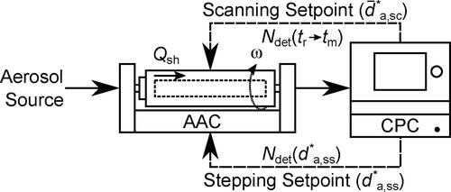
Figure 6. The experimental setup used to generate each of the four aerosols used to validate the inversion theory of the scanning AAC.

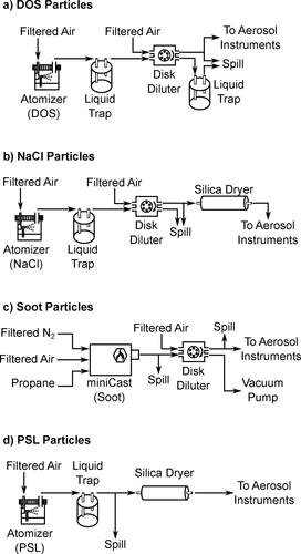
Figure 7. Comparison of particle size distributions from different aerosol sources measured by stepping or scanning the AAC, where (a) and (b) show the AAC measurements of the DOS particles at low and high classifier flows, respectively, while (c) and (d) show the AAC measurements at low classifier flows of the soot and salt particles, respectively.

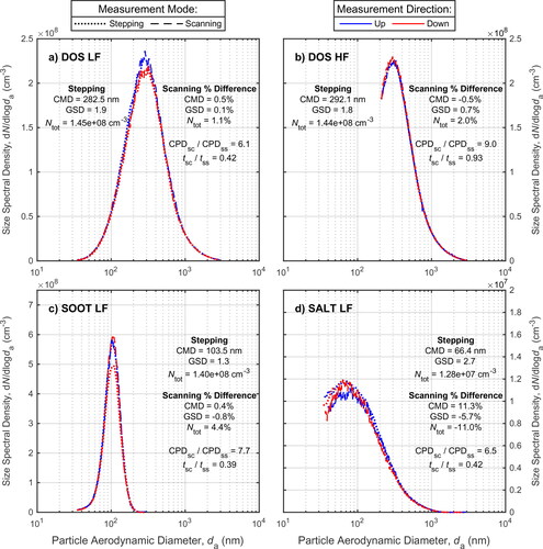
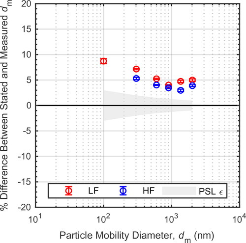
Figure 8. Agreement between PSL calibration particles and the mobility equivalent CMD of the size distribution measured by the scanning AAC. The error bars depict the repeatability of the measurements (assuming a 95% confidence interval), while the shaded region represents the uncertainty in the PSL sizes based on manufacturer specifications.