Determination of the collision rate coefficient between charged iodic acid clusters and iodic acid using the appearance time method

Figures & data

Figure 1. Example evolution of the time sequence of a single ion-induced nucleation experiment in the CLOUD chamber. The experimental conditions are 11 °C, 34% RH, 40 ppbv ozone and 8 (±6) pptv I₂ with green light on. (a) The concentrations of charged clusters are measured by an negative APi-TOF (circles joined by lines); model predictions are shown by smooth curves. They are normalized by the maximum and minimum of individual time series. The colors indicate the number of iodine atoms in the charged cluster. The chemical composition and number of iodine atoms in the charged clusters are listed in the legend with respect to colors. (b) HIO₃ concentration during the experiment. Time represents the elapsed time from the starting of the experiment in seconds.

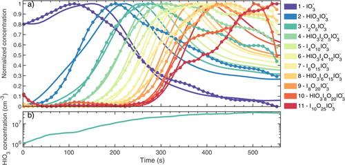
Figure 2. Schematic plot illustrating the difference between MPR/MCD and APP50 methods. The chemical composition and number of iodine atoms in the charged clusters are listed in the legend with respect to colors. u_i represents the APP50 points while u_i,M represents the MPR/MCD points.

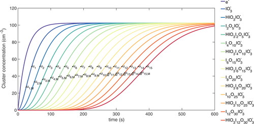
Figure 3. Comparison of the APP50, MPR and MCD methods under different experimental conditions. The y axis shows the ratio of the calculated collision rate coefficient to the model input. Different markers indicate different methods, as shown in the legend. (a) The HIO₃ concentration is 2 × 10⁷ molecules cm⁻³ and all the collision rate coefficients are set to 2 × 10⁻⁹cm³ s⁻¹. (b) The HIO₃ concentration is set to vary, the same trend as the HIO₃ concentration shown in Figure 1b. All the collision rate coefficients for odd number charged clusters are set to 2.5 × 10⁻⁹cm³ s⁻¹ and 1.5 × 10⁻⁹cm³ s⁻¹ for even number charged clusters. The missing values are negative values which the corresponding method fails to calculate.

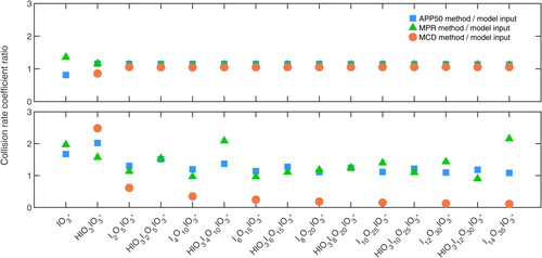
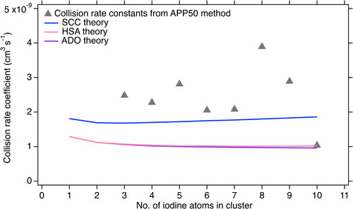
Figure 4. Collision rate coefficient calculated by the APP50 method and theoretical methods. The expected charged cluster collision rate coefficients from ADO theory are shown by the solid purple curve, values from HSA theory are shown by the solid pink line, values from the SCC method are shown by solid blue curve. The gray triangles are collision rate coefficients calculated by APP50 method based on the data shown in the Figure 1.