On aerosol formation by condensation of oil vapor in the crankcase of combustion engines

Figures & data

Figure 1. Schematic of a closed crankcase ventilation system (CCV). The blow-by flow (red arrows) contains oily aerosols. Their concentration is reduced by an oil mist separator before being vented to the intake stroke.

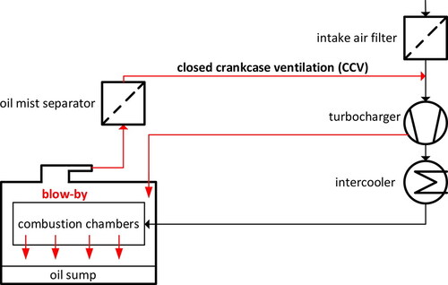
Figure 2. (a) Typical crankcase aerosol size distribution to illustrate the choice of particle size ranges. (b) Oil aerosol concentration vs. bulk oil temperature for three particle size intervals characteristic of crankcase aerosols. Data extracted from optical particle counter (OPC) measurements across a wide range of operating conditions for a medium-duty 4-cylinder 5.1-liter diesel engine. Lines inserted to guide the eye.

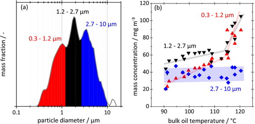
Figure 3. (a) Arrangement for sampling submicron crankcase aerosols from the crankcase of a 4-cylinder 5.1-liter diesel engine. The arrangement consists of a sampling probe, a wall-flow trap, two cyclones, and a filter to collect the aerosol. (b) Particle penetration through two cyclones connected in series. These data were obtained by OPC using a flow rate of 12.5 L/min. The compact line is a 3 point adjacent-average that serves as guide to the eyes.

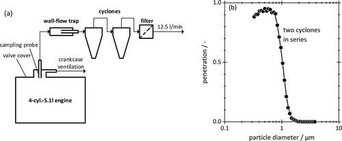
Figure 4. (a) Experimental setup used to saturate, and then, cool down a flow of vapor laden air or aerosol in a tube exposed to an ambient temperature of 25 °C. Aerosol after cool-down is characterized either by SMPS and OPC or captured on a filter for chemical analysis. (b) Gas temperature profile in the cool-down tube relative to tube inlet, here for a heating chamber temperature of 120 °C. The ambient temperature is indicated as a dashed line. The linear fit corresponds to a cooling rate of 380 K/s.

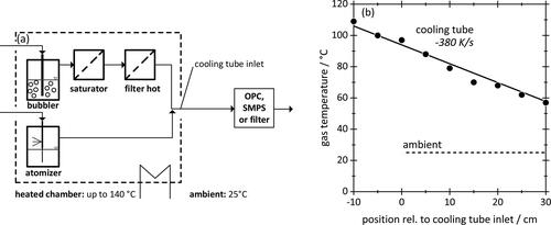
Figure 5. GC spectra of sump oil, aerosol generated from sump oil by evaporation-condensation in the lab, and crankcase aerosol from the fired engine.

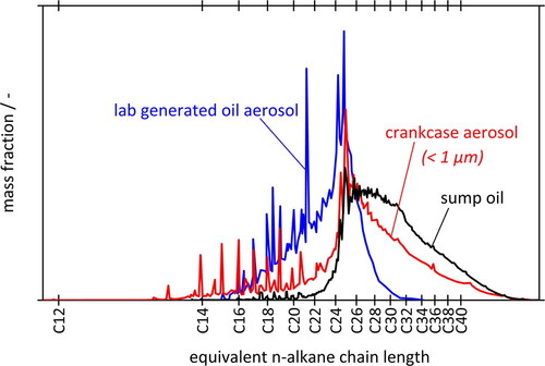
Figure 6. Equilibrium vapor concentrations for hexadecane and two engine oils. Data points are based on measurements according to Subsection 2.1. Error bars for hexadecane represent the standard deviations of three measurements each. Solid curve for hexadecane from Lemmon and Goodwin (2000); solid curves for engine oils are exponential fit functions.

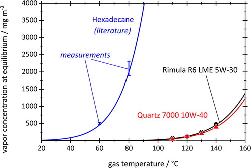
Table 1. Conditions for cool-down experiments without preexisting particles and vapor data used for simulation.

Cool-down	Material	Vapor conc. at STP	Vapor losses (%)
100 °C → 25 °C (Figure 7a)	Hexadecane	10,600 mg/m^3	99.98
110 °C → 25 °C (Figure 7b)	Hexadecane	19,000 mg/m^3	90.72
120 °C → 25 °C (Figure 8a)	Quartz 7000 10W-40	170 mg/m^3	99.67
130 °C → 25 °C (Figure 8b)	Quartz 7000 10W-40	310 mg/m^3	56.56

Figure 7. Number-based PSDs obtained by cooling down saturated particle-free hexadecane vapor from 100 °C (a) or 110 °C (b) to 25 °C. Concentrations stated at STP. OPC measurements (blue/circles) and numerical simulation (black/triangles) use the same size classes (32 logarithmically equal bins per decade).

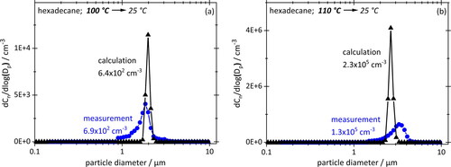
Figure 8. Number based PSDs obtained by cooling down saturated particle-free engine oil vapor from 120 °C (a) or 130 °C (b) to 25 °C. Concentrations stated at STP. SMPS measurements (blue/circles) and numerical simulation (black/triangles) use the same size classes (64 logarithmically equal bins per decade).

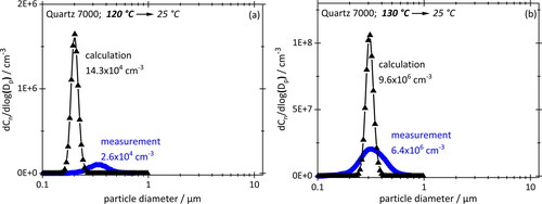
Figure 9. Simulated PSDs based (a) on number and (b) on mass for three different initial nuclei concentrations with d₀ = 30 nm. The nucleation part of the PSD shown in red (triangles), the preexisting nuclei in blue (diamonds).

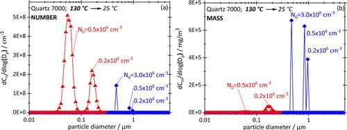
Figure 10. Measured PSDs for two concentrations N₀ of preexisting aerosol with d₀ < 600 nm. Other parameters are the same as for Figure 8.

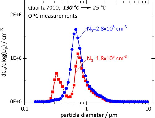
Figure 11. Total aerosol number concentrations (a) and number-weighted median particle diameters (b) plotted against gas temperature before cool-down at three different cooling rates. Equilibrium vapor concentrations and peak saturations during cool-down are added. Simulated for Quartz 7000 10W-40 with a surface tension of 30 mN/m. Lines connecting data points serve as a guide to the eye.

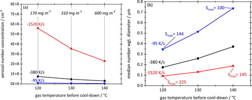
Figure 12. Total aerosol number concentrations (a) and number-weighted median particle diameters (b) plotted against gas temperature before cool-down. For each starting temperature, equilibrium vapor concentrations are scaled by factors of 0.5 (blue) and 2.0 (red) relative to the black reference curve. Actual vapor concentrations and peak saturations during cool-down have been added. Surface tension of 30 mN/m and cooling rate of –380 K/s remain unchanged. Straight lines connecting data points as a guide to the eye.

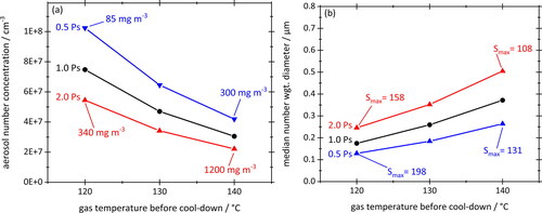
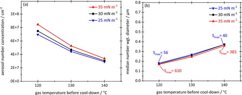
Figure 13. Total aerosol number concentrations (a) and number-weighted median particle diameters (b) plotted against the gas temperature before cool-down for three different values of surface tension. Cooling rate –380 K/s, equilibrium vapor concentration corresponding to Total Quartz 7000 10W-40. Straight lines connecting data points are a guide to the eye.