
Figures & data
Figure 1. (a) Schematic figure depicting important properties of respiratory aerosol emissions and resulting methodological challenges for sampling studies discussed in this work. (b) The size distribution of aerosol 0.3 – 500 µm diameter generated by a cough, demonstrating polydispersity in size (Johnson et al. Citation2011).
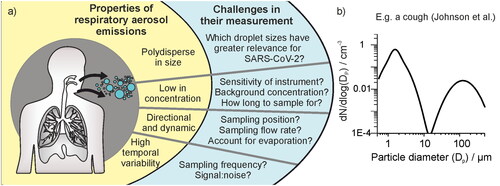
Figure 2. (a) Aerosol number concentration in a laminar flow operating theater measured with an OPS when a subject produces a voluntary cough at defined times (indicated by the blue arrows). The laminar flow in the theater is initially on, turned to standby mode at 360 s, and turned off completely at 1020 s. In both black and red data sets (two data collections), aerosol generated by a cough is clearly detected above the background concentration when the laminar flow system is on or in standby mode, but not when the laminar flow has been turned off for 8 min. (b) Expanded view of three coughs from the two data collections in a) when the laminar flow system is on standby.
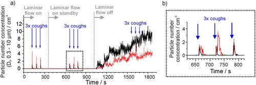
Figure 3. (a) The sampled background aerosol number concentration, (OPS, DP 0.3–10 µm), in different settings, sampled once per second for 150 samples. (b) The standard deviation from 10 s bins of the background aerosol concentration in each site shown in (a) compared to the mean concentration. (c) Allan deviation analysis on the background aerosol concentration in a chemistry lab (mean concentration ∼21 cm−3) and in an eye hospital theater (mean concentration ∼ 0.6 cm−3) compared on the same scaling to a box and whisker plot showing the number concentration generated by a cohort of 25 healthy subjects breathing, speaking or coughing (data from Gregson, Watson, et al. Citation2021). Whiskers represent the range (1.5IQR), boxes represent 25%–75% and bold line is the median concentration.
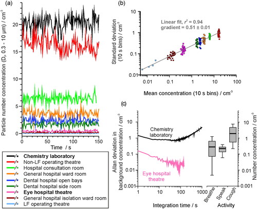
Figure 4. (a) Schematic depicting the importance of understanding the sampling flow rate relative to the exhalation rate, if sampling into a fixed volume such as a funnel, as the relationship between the two flow rates defines whether the concentration of aerosol particles or an absolute number of particles can be reported. (b) The number concentration sampled from an APS through a funnel when a subject sings at 90 – 100 dB for 10 s intervals, as the sampling flow rate is increased sequentially from 5 to 25 L min−1. (c) The number concentration sampled by an APS when a subject breathed into a funnel for 60 s, as the sampling flow rate is increased from 5 to 20 L min−1. Error bars report the standard error of the mean.
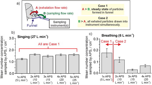
Figure 5. (a) The mean background aerosol concentration sampled within a chemistry laboratory (APS, model 3321 TSI), both when sampled once per second over 90 min (gray) or over 20 s (pink). (b) The 90-min sampled data in a represented as a histogram of likelihood of sampling a particle within a 10 s time window, for five varying particle sizes. (c)–(e) The likelihood of sampling a particle within the 1.72 µm APS size bin when sampled in (c) 10 s, (d) 20 s, or (e) 60 s sampling windows, to demonstrate the importance of sampling for a long time to gain an accurate mean concentration for particles of lower concentration. The full-width half maximum (FWHM) of the Gaussian fit (red line) is reported to show the narrowing of the distribution for longer sampling windows and the improved quantification of the particle concentration.
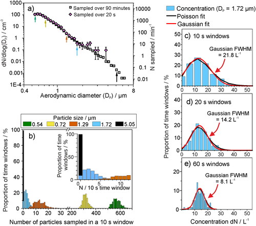
Figure 6. The size distribution of aerosol sampled by an APS in a chemistry laboratory (background concentration ∼ 20 cm−3), normalized with respect to the concentration for Dp = 1 µm, sampled over 30 min periods over a time of ∼7 h, compared with the sampled aerosol through 130 cm of conductive silicone tubing and a sampling funnel (datapoints, left axis). Lines show the cumulative fraction of aerosol generated by a cough (data from Johnson et al. Citation2011), reported in terms of number and mass concentration fraction.
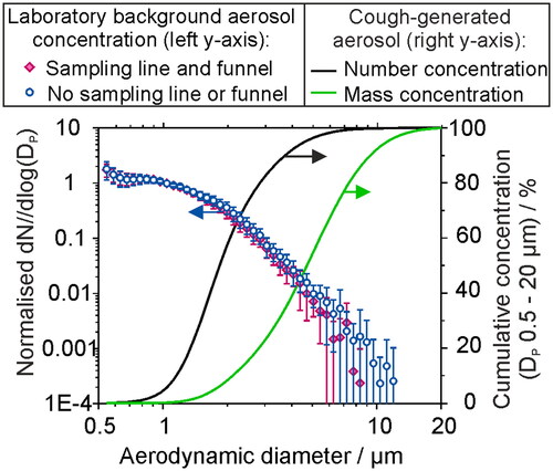
Figure 7. (a) The trajectory of a generated respiratory jet, indicating the path that aerosol droplets of respirable size (<20 µm diameter) would follow, for example flow rates to represent speech (top, 3.2 m s−1) and a cough (bottom, 15 m s−1) in an environment of 50% RH and 293 K. Positive vertical motion is in the upwards direction. (b) The simulated evaporation profiles of saliva droplets from size ranging from 0.5 – 20 µm, in conditions of 293 K and 50% RH. The hygroscopic properties of saliva are considered in the simulation. (c) The size distribution of aerosol particles generated by a cough at the source, as reported by an APS by Johnson et al., and the same plume of aerosol followed by 0.1, 0.5, and 1.0 s transit time.
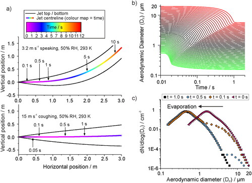
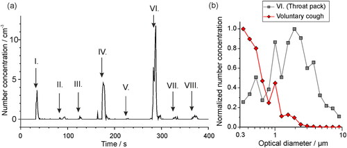
Figure 8. (a) The aerosol particle concentration detected by an OPS in a laminar flow operating theater when various different clinical materials are moved past the OPS inlet: I. Rustling green gauze, II. Rustling theater hat, III. Opening non-sterile gauze, IV. Opening sterile gauze, V. Unwrapping tracheal tube, VI. Opening throat pack, VII. Rustling fluid resistant face mask, VIII. Rubbing theater scrubs. (b) The size distribution of particles detected when a throat pack is opened near to the OPS inlet, compared to the aerosol sampled during a voluntary cough (Brown et al. Citation2020) normalized with respect to the particle size bin of largest concentration. Data are plotted from (Shrimpton, Gregson, Brown, et al. Citation2021b).
Data availability
Data are available in the BioStudies database (https://www.ebi.ac.uk/biostudies/) under accession number S-BSST718.