“Invisible bias” in the single particle soot photometer due to trigger deadtime

Figures & data

Figure 1. Left: An incandescent particle that transited the laser within the “pre-trigger number of points” (hatched area) after a triggered window—this did not generate a trigger, but the second particle (an incandescent particle at ∼ point 200) did. If the second particle did not cross the laser within this window, the first particle’s signals would not have been saved. This example was recorded from actual aerosol, and reflects the “non-paralyzable deadtime” situation. Right: synthetic data to represent the case of multiple particles crossing the laser in rapid succession, maintaining a scatter signal above threshold, and thus disabling triggering of a threshold exceedance event on the incandescent channel. The solid shaded area represents a trigger and its associated window, followed by the hatched area representing pre-trigger points beyond that window. Beyond that, deadtime is extended. This represents the “paralyzable deadtime” situation. Ambient data could not be used because in this case only the original window (solid shading) would have been saved by the SP2.

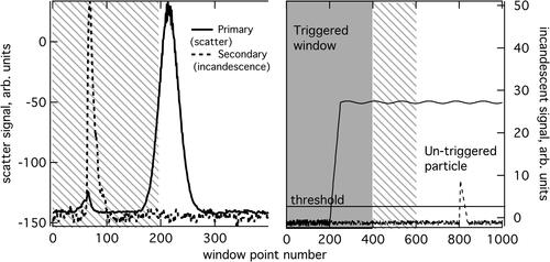
Figure 2. Trigger bias measured with rBC particles externally mixed with mono-disperse rBC-free polystyrene latex (PSL) particles using the standard SP2 configuration (DC-coupled scatter signal as primary trigger channel). Empty/solid markers are for measurements with 400 or 150 points per detection respectively. Left: Bias plotted against the rate of PSLs crossing the SP2 laser. An exponential fit is shown with the solid line. The vertical dashed line shows the nominal maximum particle rate identified by the manufacturer. Center; Bias plotted against the fraction showing evidence of excessively high particle rates (as per text). Right: Bias plotted against the average fraction of buffer-time associated with triggered windows. In this plot, markers are scaled with PSL rate (between 1000 and 150,000 s⁻¹), with larger sizes corresponding to higher rates to show that the triggered fraction decreases at the largest biases/particle rates. The straight line shows the largest magnitude bias possible for a given fraction triggered, and the dashed line is the theoretical result from Equation (3)(3) $${\mathit{B}}_{\text{rel}}=-\left({\mathit{P}}_{\text{PT}}/\mathit{T}\_\mathit{P}\right)*{\mathit{F}}_{\mathit{T}}$$(3) .

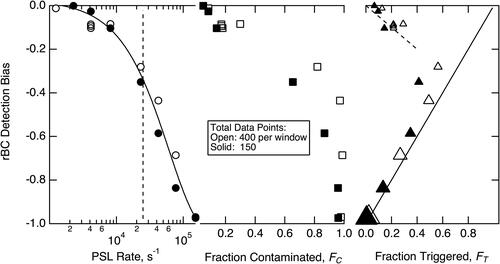
Figure 3. Bias in SP2 records of rBC particles plotted against (left) the fraction of the buffer associated with triggered windows and (right) the fraction of written windows that showed evidence of additional particle transects during the start of the window. Empty circles are for tests with relatively low rBC concentrations, and thus subject to larger relative statistical uncertainty. Filled circles were measured with high rBC concentrations and lower statistical uncertainty. The dashed line is the largest magnitude bias possible assuming that 100% of scanned windows can be associated with valid detection of an incandescent rBC-containing particle. The fits were only to high-rBC data. The fit on the left was to data <0.4 F_T and had an R² = 0.74. The fit on the right was to FC < 0.2 and had an R² of 0.6.

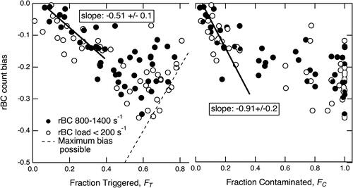
Figure 4. Exploring the impact of window length on bias. This data selected only from cases of: PSL scattering particles with AC-coupled triggering for the two extreme window lengths (150 and 400 points). Markers are sized (large = long) with window length. Left: bias plotted against scatter particle rate. Right: bias plotted against the fraction triggered, which is itself a function of both particle rate and window length. The dashed line is the simple theoretical estimate of Equation (3)(3) $${\mathit{B}}_{\text{rel}}=-\left({\mathit{P}}_{\text{PT}}/\mathit{T}\_\mathit{P}\right)*{\mathit{F}}_{\mathit{T}}$$(3) .

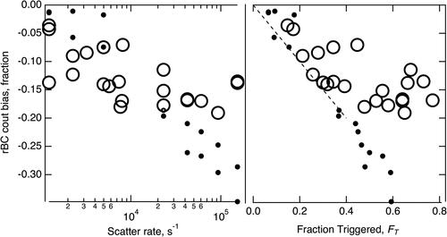
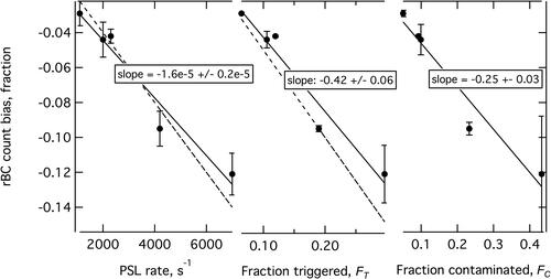
Figure 5. Relatively low-rate bias measured for 200 total data points, 100 pre-trigger points, position-sensitive detector providing primary scattering triggering. The solid lines are least-square fits to the data; the dashed lines are theoretical predictions based on Equations (1)(1) $$B_{\mathit{rel}}=\mathrm{}-R_S*\tau$$(1) and (3)(3) $${\mathit{B}}_{\text{rel}}=-\left({\mathit{P}}_{\text{PT}}/\mathit{T}\_\mathit{P}\right)*{\mathit{F}}_{\mathit{T}}$$(3) of the text.