Development of a sampling probe with a small non-isokinetic sampling error in variable flow velocity environments

Figures & data

Figure 1. Design of (a) the developed SAS probe and (b) a conventional sampling probe used in this study.

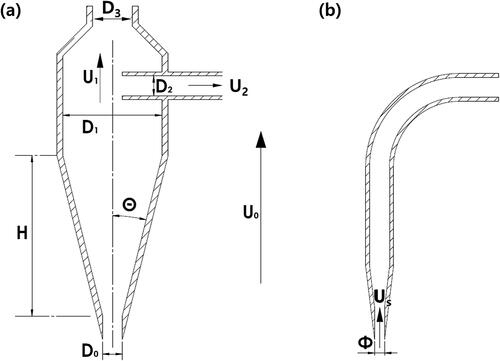
Figure 2. Schematic diagram of an experimental setup to measure particle concentrations using the SAS probe and a conventional probe with different duct flow velocities. Here, OPC is optical particle counter.

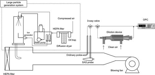
Figure 3. Sampling probe flow analysis using CFD.

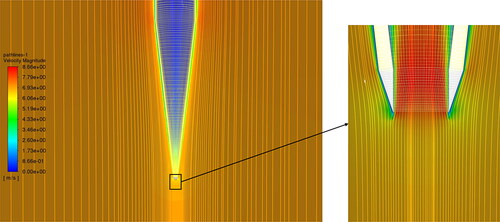
Figure 4. Particle mass concentration distributions for the SAS probe and conventional probe at isokinetic condition. The duct flow velocities (U₀) are (a) 6.4 m/s, (b) 2.8 m/s, (c) 1.6 m/s, and (d) 0.7 m/s.

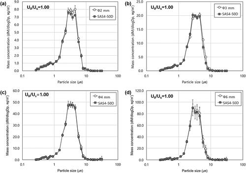
Figure 5. Particle mass concentration distributions of the conventional probe using a 4 mm nozzle (C), estimated value using Equation (5)(5) $$\frac{C}{C_0}=1+\left(\frac{U_0}{U_s}-1\right)\left(1-\frac{1}{1+\left(2+0.62U_s/U_0\right)Stk}\right).\mathrm{}$$(5) obtained based on that of the conventional probe using a 4 mm nozzle (C₀), and the developed SAS4-50D probe. The duct flow velocities are (a) 2 m/s, (b) 4 m/s, (c) 6 m/s, (d) 8 m/s, and (e) 10 m/s.

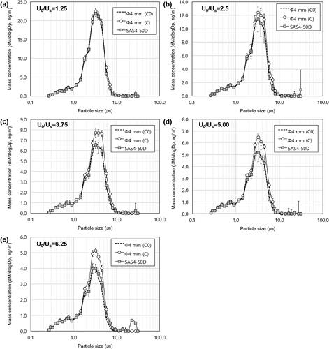
Figure 6. Particle mass concentration distributions of the conventional probe using a 2 mm nozzle (C), estimated value using Equation (5)(5) $$\frac{C}{C_0}=1+\left(\frac{U_0}{U_s}-1\right)\left(1-\frac{1}{1+\left(2+0.62U_s/U_0\right)Stk}\right).\mathrm{}$$(5) obtained based on that of the conventional probe using a 2 mm nozzle (C₀), and the developed SAS4-50D probe. The duct flow velocities are (a) 2 m/s, (b) 4 m/s, (c) 6 m/s, (d) 8 m/s, and (e) 10 m/s.

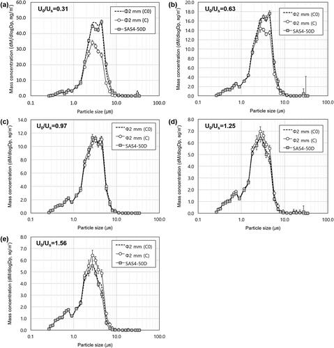
Figure 7. Particle mass concentration distributions at different sampling velocities for (a) conventional sampling probe Φ4 and (b) the developed SAS4-50D probe.

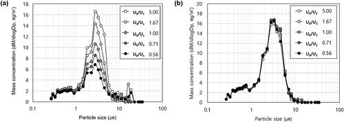
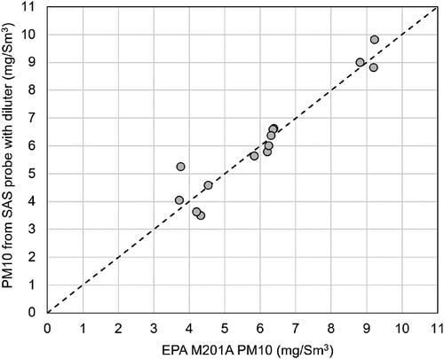
Figure 8. Comparison of the PM₁₀ concentrations measured in a stack in a coal-fired power plant in Korea obtained using the gravimetric method (EPA 201A) and the SAS probe with an ejector–porous tube dilution system.