Figures & data
Table 1. Parameters and their values used in KM-GAP simulations for a specific cooking event.
Figure 1. "Signature" emissions observed during (a) layered day 4 (b) Thanksgiving day 2. The main cooking events occurred in the middle time period shown (i.e., beef chili at 16:05-16:25 and sweet potato casserole at 14:05-14:25). The bars are clustered, with signals for all three time periods starting at zero.
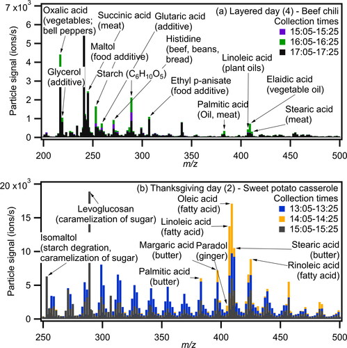
Figure 2. Distribution of measured particle-phase compounds by elemental groups: CHO, CHNO, CHClO, CHClNO, CHN, CHSO, CHNSO. The distributions are shown for (a) L3_VS: Layered day 3 – Vegetable stir fry 11:35-12:35, (b) L4_EB: Layered day 4 – English breakfast 9:05-9:25, (c) L4_VS: Layered day 4 – Vegetable stir fry 12:05-12:25, (d) L4_BC: Layered day 4 – Beef chili 16:05-16:25, (e) TG1: Thanksgiving day 1 – 14:30-15:30, (f) TG2: Thanksgiving day 2 – 14:05-14:25, (g) TG2_cat: Distribution by source category for Thanksgiving day 2 – 14:05-14:25. NOx concentrations are shown on the top panel in units of ppbv.
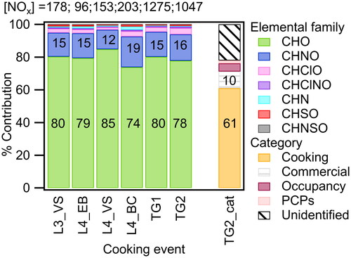
Figure 3. Aggregated signal separated by carbon and oxygen number for (a) CHO for L4_EB (b) CHNO for L4_EB (c) CHO for TG2 (14:05-14:25) (d) CHNO for TG2 (14:05-14:25). Labeled signals are for identified compounds with the highest abundance within each category.
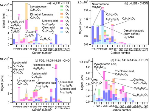
Figure 4. a) Fraction of HR-identified compounds in the particle phase versus molar mass (m/z) for TG2, particle collection period of 14:05-14:25. Compounds shown in black are all HR-identified compounds for this time-period. Compounds shown in blue are CHO-only unimodal compounds. (b) Fp of non-nitrogenated compounds in m/z region 133-163 from (a) versus their oxidation states (OSc).
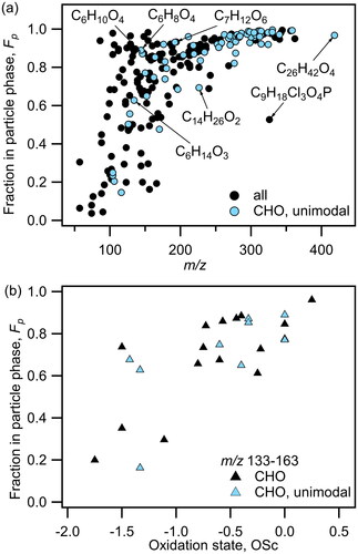
Figure 5. Fp versus m/z for a group of abundant compounds during 8 consecutive sampling periods under different OA loading conditions on TG2. Size of markers indicates magnitude of COA and their color indicates the sampling period. The solid (green) line is a fit based on 14:05-14:25 and is added to guide the eye.
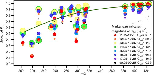
Figure 6. (a): Fp versus log(C0) obtained from Li, Pöschl, and Shiraiwa (Citation2016) correlation for two events: a high activity and a low activity period on Thanksgiving Day 2 (TG2). The black line indicates expected partitioning behavior at COA = 100 μg m3 whereas actual COA = 133.9 (b) Experimental log(C*) from FIGAERO-CIMS (calculated from Fp) versus log(C0) from Li, Pöschl, and Shiraiwa (Citation2016) parameterization based on elemental formulas of HOMEChem compounds, for seven different cooking events.
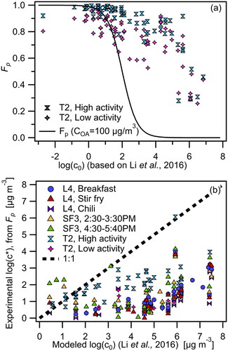
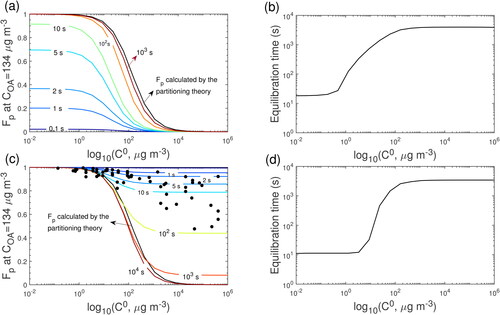
Figure 7. Predicted Fp variations with time for (a-b) condensation and (c-d) evaporation in the closed system and the Fp calculated by partitioning theory. COA is 134 μg m−3; T is 322.8 K and Db is 3 × 10⁻¹² cm2 s−1.
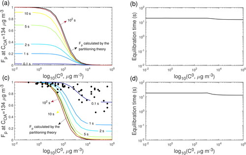
Figure 8. Predicted Fp variations with time for (a-b) condensation and (c-d) evaporation in the closed system and the Fp calculated by the partitioning theory. COA is 134 μg m−3; T is 298 K and Db is 1 × 10⁻¹⁴ cm2 s−1.