Constraining the complex refractive index of black carbon particles using the complex forward-scattering amplitude

Figures & data

Table 1. List of the publications using the BB06-h, BB06-l, and CC90 for BC refractive index.

Category	Authors and year	Research focus	BC refractive index values used/refereed
Light-scattering simulation	Moosmüller, Chakrabarty, and Arnott (2009)	Review of aerosol light absorption and its measurement techniques	BB06-h
	Kahnert and Devasthale (2011)	Spectral optical properties of pure BC aggregates	CC90
	Cheng et al. (2013)	Spectral optical properties of BC-containing particles	CC90
	Scarnato et al. (2013)	Mass absorption cross-section of NaCl-BC mixture	BB06-h
	Scarnato et al. (2015)	Spectral optical properties of a dust-BC mixture	CC90
	Wu et al. (2015)	Effect of monomer polydispersity of BC aggregates on its mass absorption cross-section	BB06-h
	Wu et al. (2018)	Morphological effects of absorption enhancement	CC90
	Beeler and Chakrabarty (2022)	Parameterization of mass absorption cross-section of BC-containing particles	BB06-h
Aerosol remote sensing	Koike et al. (2014)	Interpretation of aerosol absorption optical depth from in-situ aircraft data	BB06-h, Average of BB06-h and -l
	Schuster et al. (2016)	Distinguishing different absorbing aerosol species	BB06-h, BB06-l
	Li et al. (2019)	Retrieval of aerosol components	BB06-h, BB06-l
Aerosol-climate model	Stier et al. (2007)	Global distribution of aerosol absorption, climate model	BB06-h, BB06-l
	Zaveri et al. (2010)	Modeling aerosol’s microphysical properties, particle-resolved aerosol box model	Midpoint of BB06-h and -l
	Yu et al. (2012)	Aerosol microphysics module for climate models	Average of BB06-h and -l
	Brown et al. (2021)	Intercomparison of biomass aerosol absorption among climate models	BB06-h, BB06-l, Average of BB06-h and -l

Figure 1. Schematic diagram of the complex amplitude sensor for waterborne particles. A linearly polarized 2 mW He-Ne laser with λ = 0.633 μm was used for generating high-wavefront quality Gaussian laser beam. An optical isolator was used to prevent laser instability due to back reflections. Each pair of rotatable half-wave plates (HWPs) with polarization beam splitters (PBSs) was used to split the beam with a controlled power ratio. The beam optics in the s- and l-channels are configured to quantify the complex forward-scattering amplitude of the sub- and super-micron particle size range, respectively. Table S1 lists the models and manufacturers of all the optical components in this schematic.

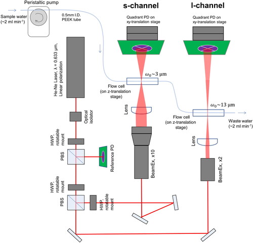
Figure 2. Examples of the geometric arrangement of spherical monomers in the AGGREGATE and SPHPACK models. (a) AGGREGATE with fractal dimension 2.0, (b) AGGREGATE with fractal dimension 2.5, (c) SPHPACK with packing density 0.05, (d) SPHPACK with packing density 0.30. The number of monomers N_pp is 1024 in each example. The length unit of each Cartesian coordinate is the monomer radius.

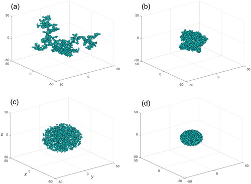
Table 2. List of the particle shape models and their parameters (r_v, m_r, m_i, θ_s).

Shape model	Morphology	Model constants	Number of monomers	Volume equivalent radius $r_{\mathrm{v}}$	Real part of refractive index $m_{\mathrm{r}}$	Imag. part of refractive index $m_{\mathrm{i}}$	Shape parameter ${\theta }_s$
AGGREGATE	A fractal-like aggregate of spherical monomers	Monomer radius rpp = 0.030 μm, Fractal prefactor kf = 1.0	Npp = 2^2, 2^3, …, 2^14	0.048–0.76 μm, 13 grid points in log space	1.4–3.3, 20 grid points in linear space	0.0–1.5, 16 grid points in linear space	Fractal dimension 2.0–2.5 6 grid points in linear space
SPHPACK	Randomly positioned non-overlapping spherical monomers within a spherical volume	Monomer radius rpp = 0.030 μm					Packing density 0.05–0.3 6 grid points in linear space

Figure 3. Flow chart of the computational and data processing procedure in our method for constraining the refractive index of ambient BC from the complex forward-scattering amplitude measurements. The frame color shows either of data, forward model, or Bayesian probability as illustrated in the lower-left part of the Figure.

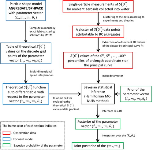
Figure 4. Typical examples of transmission electron microscope (TEM) images of laboratory powder samples. (a) Fullerene soot, (b) BC aggregate in the Vehicle exhaust particulates, (c) Hematite-KJ, and (d) Hematite-TD. The TEM images were obtained using a 120-kV TEM (JEM-1400, JEOL).

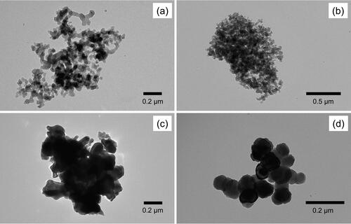
Table 3. List of the laboratory test samples.

Sample name	Chemical composition	Supplier and product number	Morphology of individual particles from TEM images
Fullerene Soot	Synthetic BC powder consisting of aggregates of ns-soot nanoparticles	Alfa Aesar, Inc. Stock# 40971, Lot#FS12S011	Compact aggregate of near-spherical nanoparticles with monomer diameter ∼20–50 nm. Essentially all the attached monomer pairs are sintered.
Vehicle Exhaust Particulates	Reference material extracted from vehicle exhaust. The BC mass fraction of this powder was estimated to be ∼80% (Honda 2021)	National Institute of Environmental Studies, Japan. Certified Reference Material No.8: Vehicle Exhaust Particulates.	Compact aggregate of near-spherical nanoparticles with monomer diameter ∼10–40 nm. Most of the attached monomer pairs are weakly sintered.
Hematite-KJ	Synthetic hematite powder consisting of aggregate of α-Fe2O3 nanoparticles	Kojundo Chemical Laboratory Co. Ltd., FEO14PB, 99.9% purity, c.a. 0.3 μm	Compact aggregate of nonspherical nanoparticles with monomer maximum dimension < ∼100 nm. Essentially all the attached monomer pairs are strongly sintered.
Hematite-TD	Synthetic hematite powder consisting of aggregate of α-Fe2O3 nanoparticles	Toda Kogyo Co. Lot# 180611 Specific surface area = 10.5 m^2g^−1	Compact aggregate of near-spherical nanoparticles with monomer diameter ∼30–100 nm. Most of the attached monomer pairs are not sintered.

Figure 5. Typical examples of transmission electron microscope (TEM) images of ambient aerosols collected by an aerosol-impactor sampler installed on the research vessel SHINSEI MARU. Each panel shows samples collected around 12:00 local time on (a) July 27^th, (b) July 28^th, (c) July 30^th, and (d) August 1^st. Red arrows indicate individual BC aggregates, most of which were mixed with sulfate (green arrows) and/or organics (light blue arrows). The TEM images were obtained using a 120-kV TEM (JEM-1400, JEOL).

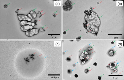
Figure 6. Scatterplot of the complex forward-scattering amplitude obtained for each of the laboratory powder samples suspended in water. Black dots show raw single particle S(0°) data. The red-filled circles show the 0^th, 5^th, …, and 100^th percentiles of the arclength coordinate of the principal curve. These 21 data points were used as the observation data vector for Bayesian inference. The red circles are concentrated in proportion to the local density of raw data points.

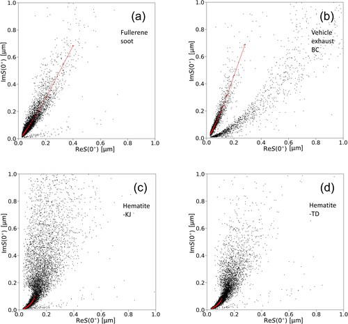
Figure 7. Same plots as Figure 6 but for atmospheric water-insoluble aerosols collected into water on each of the 6 observation days. Principal curve fit was applied to the linear-shape cluster of data points with ImS(0°)/ReS(0°) > ∼1, which is attributable to BC aggregates.

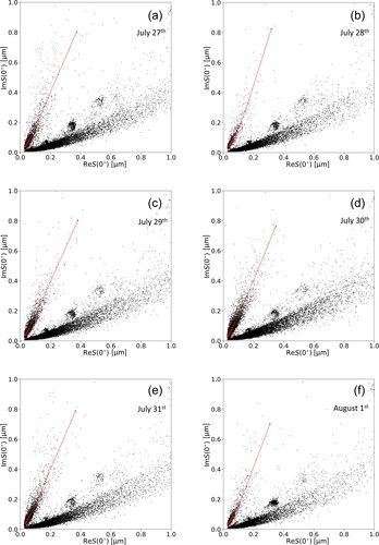
Figure 8. Posterior of real and imaginary parts of complex refractive index (m_r, m_i) for each laboratory sample derived from the data shown in Figure 6. (a) Fullerene soot, (b) Vehicle exhaust BC, (c) Hematite-KJ, (d) Hematite-TD. The three-level contour shows the 90%, 50%, and 10% highest density credibility regions for each of the AGGREGATE (green) and SPHPACK (blue) models. Marginalized density distributions of m_r and m_i are also shown along horizontal and vertical axes, respectively. In each panel, the BB06-l and -h values were also shown by gray-filled circles for comparison. In panels (a) and (b), the SPHPACK is more realistic shape model than the AGGREGATE for the reasons explained in the main text.

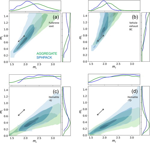
Figure 9. Same plot as Figure 8 but for atmospheric BC results derived from the data shown in Figure 7. In each panel, the BB06-l and -h values were also shown by gray-filled circles for comparison. The dashed lines indicate the boundary of our suggested plausible (m_r, m_i) domain for atmospheric BC, which approximate the 90% highest density credibility regions. The SPHPACK is more realistic shape model than the AGGREGATE for the reasons explained in the main text.

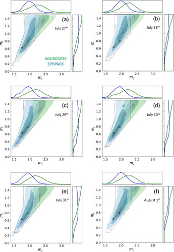
Figure 10. Joint density plots of the posteriors of real and imaginary parts of refractive index, m_r, m_i, and the two volume-equivalent radii corresponding to the 95^th and 100^th percentiles of arclength coordinate of the principal curve, r_v95, r_v100 for atmospheric BC sampled on August 1^st. The three-level contour shows the 90%, 50%, and 10% highest density credibility regions in each of the AGGREGATE (green) and SPHPACK (blue) models. The SPHPACK is more realistic shape model than the AGGREGATE for the reasons explained in the main text.

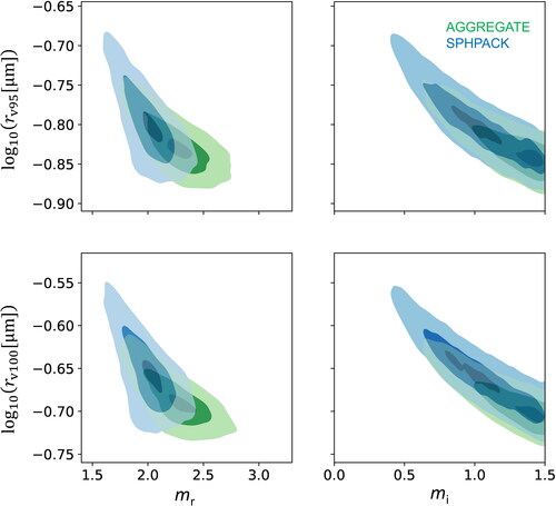
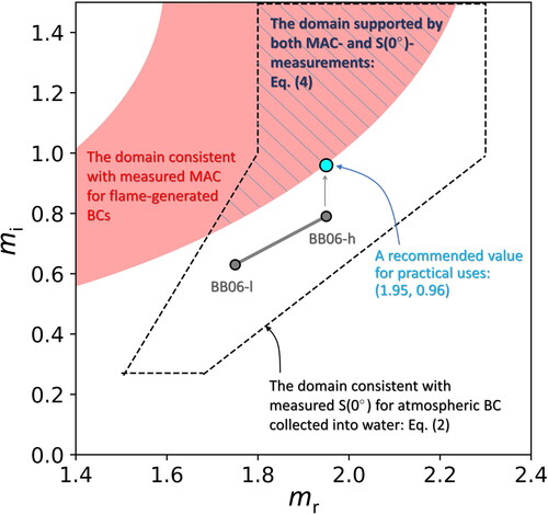
Figure 11. Illustrating the three-different (m_r, m_i) domains for complex refractive index of BC: 1) a domain consistent with measured S(0°) for atmospheric BC (enclosed by black-dashed lines), 2) a domain consistent with measured MAC for various flame-generated BCs (red-filled area), and 3) a domain supported by both MAC- and S(0°)-measurements. The conventional assumptions BB06-l (1.75 + 0.63i) and -h (1.95 + 0.79i) (gray filled circles), and our recommendable value for practical uses 1.95 + 0.96i (blue-filled circle) are also plotted.

Moosmüller, H., R. K. Chakrabarty, and W. P. Arnott. 2009. Aerosol light absorption and its measurement: A review. J. Quant. Spectrosc. Radiat. Transf. 110 (11):844–78. doi:10.1016/j.jqsrt.2009.02.035.

 Web of Science ®Google Scholar

Kahnert, M., and A. Devasthale. 2011. Black carbon fractal morphology and short-wave radiative impact: A modelling study. Atmos. Chem. Phys. 11 (22):11745–59. doi:10.5194/acp-11-11745-2011.

 Web of Science ®Google Scholar

Cheng, T., X. Gu, Y. Wu, H. Chen, and T. Yu. 2013. The optical properties of absorbing aerosols with fractal soot aggregates: Implications for aerosol remote sensing. J. Quant. Spectrosc. Radiat. Transf. 125:93–104. doi:10.1016/j.jqsrt.2013.03.012.

 Web of Science ®Google Scholar

Scarnato, B. V., S. Vahidinia, D. T. Richard, and T. W. Kirchstetter. 2013. Effects of internal mixing and aggregate morphology on optical properties of black carbon using a discrete dipole approximation model. Atmos. Chem. Phys. 13 (10):5089–101. doi:10.5194/acp-13-5089-2013.

 Web of Science ®Google Scholar

Scarnato, B. V., S. China, K. Nielsen, and C. Mazzoleni. 2015. Perturbations of the optical properties of mineral dust particles by mixing with black carbon: A numerical simulation study. Atmos. Chem. Phys. 15 (12):6913–28. doi:10.5194/acp-15-6913-2015.

 Web of Science ®Google Scholar

Wu, Y., T. Cheng, L. Zheng, and H. Chen. 2015. A study of optical properties of soot aggregates composed of poly-disperse monomers using the superposition T-matrix method. Aerosol Sci. Technol. 49 (10):941–9. doi:10.1080/02786826.2015.1083938.

 Web of Science ®Google Scholar

Wu, Y., T. Cheng, D. Liu, J. D. Allan, L. Zheng, and H. Chen. 2018. Light absorption enhancement of black carbon aerosol constrained by particle morphology. Environ. Sci. Technol. 52 (12):6912–9. doi:10.1021/acs.est.8b00636.

 PubMed Web of Science ®Google Scholar

Beeler, P., and R. K. Chakrabarty. 2022. Constraining the particle-scale diversity of black carbon light absorption using a unified framework. Atmos. Chem. Phys. 22 (22):14825–36. doi:10.5194/acp-22-14825-2022.

 Web of Science ®Google Scholar

Koike, M., N. Moteki, P. Khatri, T. Takamura, N. Takegawa, Y. Kondo, H. Hashioka, H. Matsui, A. Shimizu, and N. Sugimoto. 2014. Case study of absorption aerosol optical depth closure of black carbon over the East China Sea. J. Geophys. Res. Atmos. 119 (1):122–36. doi:10.1002/2013JD020163.

 Web of Science ®Google Scholar

Schuster, G. L., O. Dubovik, and A. Arola. 2016. Remote sensing of soot carbon–Part 1: Distinguishing different absorbing aerosol species. Atmos. Chem. Phys. 16 (3):1565–85. doi:10.5194/acp-16-1565-2016.

 Web of Science ®Google Scholar

Li, L., O. Dubovik, Y. Derimian, G. L. Schuster, T. Lapyonok, P. Litvinov, F. Ducos, D. Fuertes, C. Chen, Z. Li, et al. 2019. Retrieval of aerosol components directly from satellite and ground-based measurements. Atmos. Chem. Phys. 19 (21):13409–43. doi:10.5194/acp-19-13409-2019.

 Web of Science ®Google Scholar

Stier, P., J. H. Seinfeld, S. Kinne, and O. Boucher. 2007. Aerosol absorption and radiative forcing. Atmos. Chem. Phys. 7 (19):5237–61. doi:10.5194/acp-7-5237-2007.

 Web of Science ®Google Scholar

Yu, F., G. Luo, and X. Ma. 2012. Regional and global modeling of aerosol optical properties with a size, composition, and mixing state resolved particle microphysics model. Atmos. Chem. Phys. 12 (13):5719–36. doi:10.5194/acp-12-5719-2012.

 Web of Science ®Google Scholar

Brown, H., X. Liu, R. Pokhrel, S. Murphy, Z. Lu, R. Saleh, T. Mielonen, H. Kokkola, T. Bergman, G. Myhre, et al. 2021. Biomass burning aerosols in most climate models are too absorbing. Nat. Commun. 12 (1):277. doi:10.1038/s41467-020-20482-9.

 PubMed Web of Science ®Google Scholar

Honda, M. 2021. Multielement quantification and Pb isotope analysis of the certified reference material ERM-CZ120 for fine particulate matter. Geochem. J. 55 (6):355–71. doi:10.2343/geochemj.2.0642.

 Web of Science ®Google Scholar

Code availability

The originally developed Python module used for auto-differentiable multidimensional spline interpolation of gridded data is available from: https://github.com/nmoteki/ndimsplinejax. The code used for generating fractal-like aggregates of spheres is available from https://github.com/nmoteki/aggregate_generator. Other codes used for this study are available from the corresponding author upon reasonable request.

Data availability statement

Data generated for Figures 6 and 7 are available from: https://doi.org/10.5281/zenodo.7478889.