1,696
Views
9
CrossRef citations to date
0
Altmetric
Original Articles

Evaluation of Continuous and Filter-Based Methods for Measuring PM2.5 Mass Concentration

, , &
Pages 290-303 | Received 17 Mar 2004, Accepted 24 Jan 2005, Published online: 23 Feb 2007

Figures & data

Table 1 Sampler configuration of continuous and integrated samplers used for PM2.5 mass measurements in Houston and Seattle

Table 2 Sampler characteristics and sampling information for PM2.5 speciation instruments used in the study

Figure 1 Variation of hourly PM2.5 mass collected using continuous instruments and scattering coefficients measured in Houston, TX. The RAMS values plotted were adjusted by a factor of 1.52.
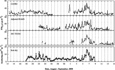
Figure 1 Variation of hourly PM2.5 mass collected using continuous instruments and scattering coefficients measured in Houston, TX. The RAMS values plotted were adjusted by a factor of 1.52.

Table 3 Mean concentration (μg m−3) of valid hourly PM2.5 mass during the measurement period

Figure 2 Variation of hourly PM2.5 mass collected using continuous instruments and scattering coefficients measured in Seattle, WA.
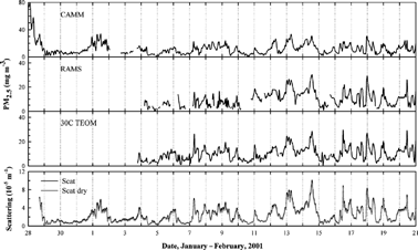
Figure 2 Variation of hourly PM2.5 mass collected using continuous instruments and scattering coefficients measured in Seattle, WA.

Figure 3 Intercomparison of 1 h average continuous PM2.5 mass measurements in Houston. The solid lines are the Deming linear regression fits in .
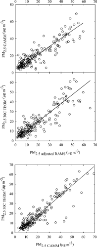
Figure 3 Intercomparison of 1 h average continuous PM2.5 mass measurements in Houston. The solid lines are the Deming linear regression fits in Table 4.

Table 4 Deming slopes and intercepts for PM2.5 mass between pairs of the continuous mass samplersFootnote a

Figure 4 Intercomparison of 1 h average continuous PM2.5 mass measurements in Seattle. The solid lines are the Deming regression fits in .
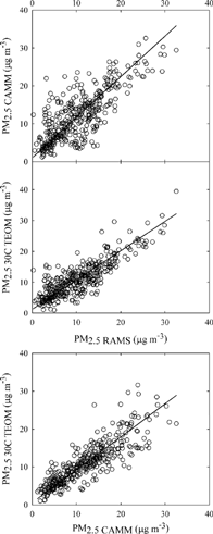
Figure 4 Intercomparison of 1 h average continuous PM2.5 mass measurements in Seattle. The solid lines are the Deming regression fits in Table 4.

Figure 5 Difference between the adjusted RAMS and 30°C TEOM mass with RH and T in Houston.

Figure 5 Difference between the adjusted RAMS and 30°C TEOM mass with RH and T in Houston.

Figure 6 Comparison of 24 h average continuous PM2.5 mass and integrated PM2.5 mass concentrations in Houston: Daily variation of PM2.5 mass (top) and standard linear regressions (bottom). The solid lines are the standard regression fits.
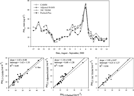
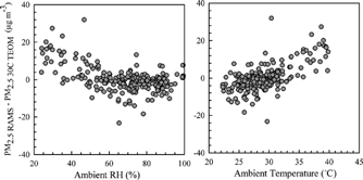
Figure 6 Comparison of 24 h average continuous PM2.5 mass and integrated PM2.5 mass concentrations in Houston: Daily variation of PM2.5 mass (top) and standard linear regressions (bottom). The solid lines are the standard regression fits.
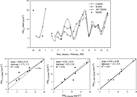
Table 5 Average concentration (μg m−3) of PM2.5 mass and species measured from the continuous and integrated samplers in Houston

Figure 7 Comparison of 24 h average continuous PM2.5 mass and integrated PM2.5 mass concentrations in Seattle: Daily variation of PM2.5 mass (top) and standard linear regressions (bottom). The solid lines are the standard regression fits.

Figure 7 Comparison of 24 h average continuous PM2.5 mass and integrated PM2.5 mass concentrations in Seattle: Daily variation of PM2.5 mass (top) and standard linear regressions (bottom). The solid lines are the standard regression fits.

Reprints and Corporate Permissions

Please note: Selecting permissions does not provide access to the full text of the article, please see our help page How do I view content?

To request a reprint or corporate permissions for this article, please click on the relevant link below:

Academic Permissions

Please note: Selecting permissions does not provide access to the full text of the article, please see our help page How do I view content?

Obtain permissions instantly via Rightslink by clicking on the button below:

If you are unable to obtain permissions via Rightslink, please complete and submit this Permissions form. For more information, please visit our Permissions help page.