714
Views
6
CrossRef citations to date
0
Altmetric
Original Articles

Use of Numerical Calculations to Simulate the Sampling Efficiency Performance of a Personal Aerosol Sampler

Pages 596-610 | Received 08 Mar 2005, Accepted 10 May 2005, Published online: 23 Feb 2007

Figures & data

Table 1 Cell numbers used in computational grids

Table 2 Low- and high-level coding map for parameter space analysis

Figure 1 Upper left: Photo of GSP sampler. Upper right: Dimensions of Computational Test Aerosol Sampler, surface mesh is for illustrative purposes. Bottom: Layout of Computational Aerosol Sampler, Reference Probe, Ideal Sampling Faces, and Particle Release Locations.
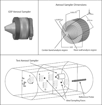
Figure 1 Upper left: Photo of GSP sampler. Upper right: Dimensions of Computational Test Aerosol Sampler, surface mesh is for illustrative purposes. Bottom: Layout of Computational Aerosol Sampler, Reference Probe, Ideal Sampling Faces, and Particle Release Locations.

Table 3 Values determined from parameter space analysis to yield 10% or greater influence on desired results are shown in bold

Figure 2 Plotted uncertainties determined from grid convergence studies on three grid densities of simulation results of the test aerosol sampler and the reference probe sampler at 0.5 and 1 m/s wind speeds for the 0-degree orientation.
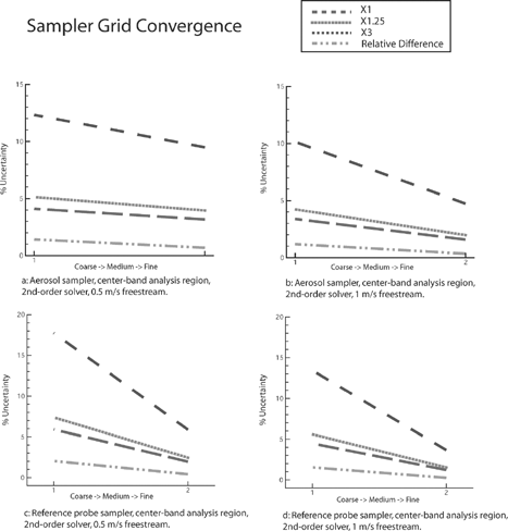
Figure 2 Plotted uncertainties determined from grid convergence studies on three grid densities of simulation results of the test aerosol sampler and the reference probe sampler at 0.5 and 1 m/s wind speeds for the 0-degree orientation.

Figure 3 Scalar values for center-band comparison region at the inlet of the GSP sampler plotted against increasing grid density.
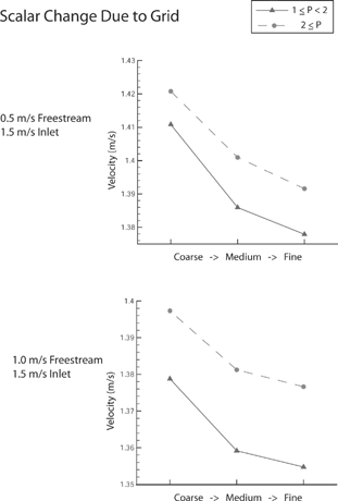
Figure 3 Scalar values for center-band comparison region at the inlet of the GSP sampler plotted against increasing grid density.

Figure 4 Computational surface mesh and grid elements on inside and outside surfaces of test aerosol sampler for nonconforming turbulent y + values tagged for adaption. Box: 2D slice of inlet cells before and after adaption.
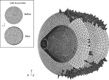
Figure 4 Computational surface mesh and grid elements on inside and outside surfaces of test aerosol sampler for nonconforming turbulent y + values tagged for adaption. Box: 2D slice of inlet cells before and after adaption.

Figure 5 Sampling efficiency of sharp-edged probe sampler from FLUENT calculations at freestream velocities of 0.5 and 1.0 m/s.
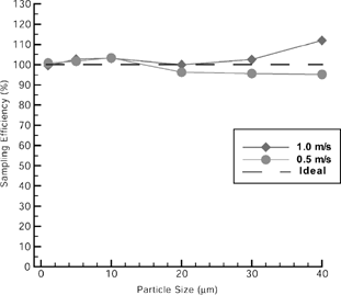
Figure 5 Sampling efficiency of sharp-edged probe sampler from FLUENT calculations at freestream velocities of 0.5 and 1.0 m/s.

Table 4 Calculated and corrected “filter-only” sampling efficiencies from CFD simulation of the test aerosol sampler free in the air in 0.5 m/s freestream airflow with corresponding experimental data from the CIS sampler (CitationLi 1999)

Table 5 Calculated and corrected “filter-only” sampling efficiencies from CFD simulation of the test aerosol sampler free in the air in 1 m/s freestream airflow with corresponding experimental data from the CIS sampler (CitationLi 1999)

Reprints and Corporate Permissions

Please note: Selecting permissions does not provide access to the full text of the article, please see our help page How do I view content?

To request a reprint or corporate permissions for this article, please click on the relevant link below:

Academic Permissions

Please note: Selecting permissions does not provide access to the full text of the article, please see our help page How do I view content?

Obtain permissions instantly via Rightslink by clicking on the button below:

If you are unable to obtain permissions via Rightslink, please complete and submit this Permissions form. For more information, please visit our Permissions help page.