Figures & data
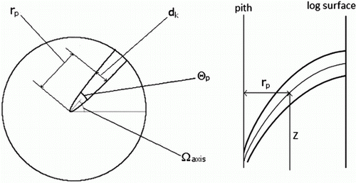
Figure 1. Description of the key geometrical features for SPSB knots. These features are calculated using the 11 Swedish Pine Stem Bank knot parameters A–K.

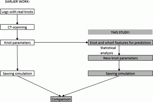
Figure 2. Description of the main structure of this study. Note the distinction between the physical knots in the log, the knots as represented in the Swedish Pine Stem Bank by parameters, and the knot features used for reconstructing the knots. Furthermore, at the last step the sawing simulation is made on the same set of physical knots, but reconstructed in two separate ways. The original SPSB knots (left) are considered ground truth and are the foundation for the new parameterisation of the SPSB knots (right).

Table I. Features used for reconstructing knots. These features are possible to extract using two-directional X-ray scanning, and in this study were calculated for the SPSB knots.
Table II. Number of whorls with different knot frequencies, according to the definition used in this study. The sets of data in the two rows are both from the Swedish Pine Stem Bank; the first row is the number of whorls obtained with the above method, the second row is the number of whorls obtained by a method used in an earlier study by Björklund (Citation1997).
Figure 3. Reconstruction of knot parameters, from measurable log properties. From the features ▵Height, WhorlHeight, Whorl volume and SurfaceDist, each whorl is reconstructed (i.e. number of knots in the whorl and a typical pattern for cardinal direction of the knots). The individual knots are finally modelled in a parametric fashion from the whorl features. Note: solid arrows denote direct or linear relations; dashed arrows denote models with some sort of random element involved. K f =number of knots per whorl, A–K=SPSB knot parameters. Darkest area: knot features/parameters, semi-dark area: whorl features, light area: features from the SPSB. The numbers represent the different steps in the overall model, numbered 1–4.

Table III. Sawn timber prices used in this study.
Figure 4. Three examples of typical whorl patterns, from the Swedish Pine Stem Bank, for whorls with four knots. This figure shows the cross-sectional view of a log, seen from the top end. Note: The zero-degree direction corresponds to north in the standing tree. Each straight line corresponds to the cardinal direction, at the pith, of a knot. The uppermost right degree-interval limits the direction of the first knot, clock-wise, from the northern direction. All other degree-intervals limit the angular distances between knots.

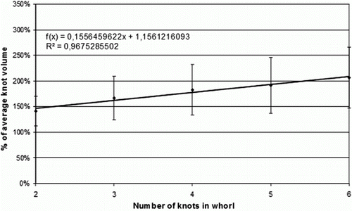
Figure 5. The largest knot's percentage of the average knot volume, plotted against number of knots in the whorl. The vertical lines show the distance of one standard deviation around the average.

Table IV. Models for reconstructing knot parameters from the knot volume (V). Note that the models for parameters H, J and dead knot percentage were not used in the final method.
Table V. Comparison of the grades assigned to boards which have knots reconstructed by the method described, and the original SPSB knots.
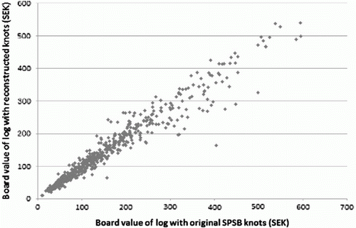
Figure 6. Simulated value of logs with reconstructed knots, plotted against the simulated value of logs with the original SPSB knots; values in Swedish Crowns (SEK).
