Abandoning conversion from even-aged to uneven-aged forest stands – the effects on production and economic returns

Figures & data

Figure 1. Location of the inventoried stands used as input to the simulation. The three clusters of stands were located in northern (9 stands), central (5 stands) and southern Sweden (10 stands).

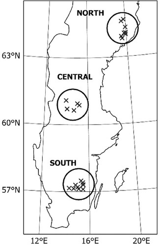
Table 1. Stand characteristics of the inventoried regenerations used as input to the simulations. Height is the arithmetic mean tree height. Height and tree species distribution refers to the total number of stems.

								Tree species distribution (%)
Region	No. of stands		Site index	Age (yr)	No. of spruce trees ha^−1	Total no. of trees ha^−1	Height (m)	Spruce	Pine	Birch	Other
North	9	Mean	17.9	9.4	2500	24,100	0.9	14	5	49	31
		Min	14.3	9	1100	6800	0.7	5	1	10	0
		Max	20.8	10	4600	39,700	1.3	25	14	75	81
		SD	2	0,5	1000	9500	0.2	7	5	25	26
Central	5	Mean	24.1	8.8	1500	5700	1.1	30	26	33	11
		Min	21.5	8	800	4700	0.8	18	2	10	0
		Max	25.6	9	1900	7300	1.2	43	41	44	35
		SD	1.6	0.4	400	1100	0.2	10	15	14	15
South	10	Mean	29	6.9	3700	19,800	1.1	25	10	52	13
		Min	24.7	6	2100	6600	0.8	14	1	25	1
		Max	31.8	7	6100	30,000	1.5	51	23	71	43
		SD	2.2	0.3	1500	7300	0.2	11	7	15	12

Figure 2. The structure of the scenario simulation. Pre-commercial thinning aimed at leaving larger trees (PCTBAU), a uniform distribution (PCTU) or an inverse J-shaped distribution (PCTJ). The scenarios simulated in Heureka were traditional management (BAU) with two commercial thinnings (CT 1, CT 2) and clear felling, conversion to selection forestry (SF) initiated at PCT (CPCTJ, CPCTU) or at the time of first (CT1) or second (CT2) commercial thinning in BAU. Scenarios for basal area after thinning were 75% (T75) and 60% (T60) compared to conventional guidelines (Skogsstyrelsen 1985a, 1989). Scenarios for abandonment of conversion forestry was continuous SF and clear felling at the same age as in BAU (ABAU), ending SF at minimum cutting age according to Swedish forestry act (SFA) and clear felling at max LEV (AEarly) and ending SF at minimum cutting age +20 years and clear felling at max LEV (ALate).

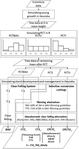
Figure 3. Diameter distribution after different conversion treatments at pre-commercial thinning (PCT). The distribution is presented for each stand (grey line) and as an average for each region (black solid line). In addition, the average diameter distribution after traditional PCT (black dashed line) is presented as a reference. The frequency refers to the relationship between the stem number in each class and the total number of stems. Average skewness (S) and kurtosis (K) is presented for each treatment and region. For abbreviations of PCT alternatives, see Figure 2.

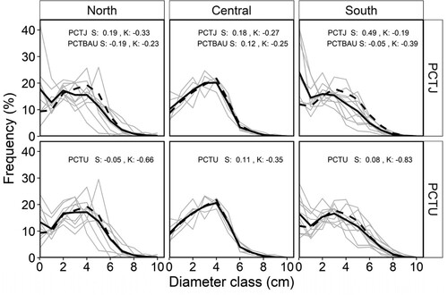
Figure 4. Diameter distribution for each region and conversion strategy at the time of final felling in abandonment scenario ABAU. Average (black solid line) and stand-wise (grey solid line) distributions are presented for selection cutting scenarios T60. Average distribution is also presented for selection cutting scenarios T75 (dashed line) and traditional BAU (dotted line). The frequency refers to the proportion of the total stem number within each diameter class. For abbreviations of conversion strategies, see Figure 2.

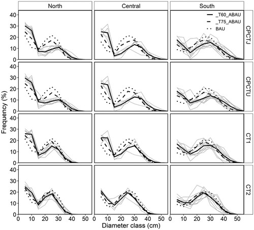
Table 2. Characteristics of thinnings, selection cuttings and rotation length for each scenario, abandonment option and interest rate over the period from start of simulation to time of final felling. Average is presented for number of conventional thinnings or selection cuttings (N), basal area before (B_bef, m² ha⁻¹) and after (B_aft, m² ha⁻¹) removal and rotation length (RL, year). For abbreviations of scenarios and abandonment options, see Figure 2.

						Interest rate (%)
						1				2				3
	Rel.	Aband.	Conventional thinnings			Sel. thinnings				Sel. thinnings				Sel. thinnings
Strategy	TG	timing	N	Bbef	Baft	N	Bbef	Baft	RL	N	Bbef	Baft	RL	N	Bbef	Baft	RL
BAU			2	31	24				95				84				77
CPCTJ	_T60	_AEarly				3.6	21	13	88	3.6	21	13	84	3.6	21	13	78
CPCTU						3.5	21	14	88	3.5	21	14	82	3.5	21	14	78
CT1						3.0	26	16	93	3.0	26	16	86	3.0	26	16	79
CT2			1	28	22	1.2	33	20	96	1.2	33	20	88	1.2	33	20	77
CPCTJ	_T75	_AEarly				2.9	25	17	95	2.9	25	17	86	2.9	25	17	77
CPCTU						2.9	25	17	93	2.9	25	17	85	2.9	25	17	75
CT1						2.8	28	19	96	2.8	28	19	85	2.8	28	19	77
CT2			1	28	22	1.2	33	23	96	1.2	33	23	86	1.2	33	23	76
CPCTJ	_T60	_ALate				5.3	21	14	100	5.3	21	14	100	5.3	21	14	99
CPCTU						5.1	21	14	96	5.1	21	14	96	5.1	21	14	96
CT1						4.5	24	16	97	4.5	24	16	96	4.5	24	16	96
CT2			1	28	22	2.9	28	18	97	2.9	28	18	96	2.9	28	18	94
CPCTJ	_T75	_ALate				4.5	25	18	98	4.5	25	18	96	4.5	25	18	96
CPCTU						4.5	26	19	97	4.5	26	19	96	4.5	26	19	96
CT1						4.2	27	20	96	4.4	25	17	95	4.2	27	20	94
CT2			1	28	22	2.6	31	22	97	2.6	31	22	92	2.6	31	22	91
CPCTJ	_T60	_ABAU				5.0	21	14	95	4.2	21	14	84	3.8	21	13	77
CPCTU						5.0	21	14	95	4.2	21	14	84	3.8	21	14	77
CT1						4.4	24	16	95	3.6	25	16	84	3.0	25	16	77
CT2			1	28	22	2.9	28	18	95	2.2	30	18	84	1.6	32	19	77
CPCTJ	_T75	_ABAU				4.4	25	18	95	3.6	25	18	84	3.3	25	17	77
CPCTU						4.4	26	18	95	3.7	25	18	84	3.4	25	18	77
CT1						4.0	27	20	95	3.5	27	20	84	2.9	28	19	77
CT2			1	28	22	2.8	31	22	95	2.1	32	22	84	1.6	33	23	77

Figure 5. Mean annual volume growth for different abandonment options AEarly (black), ALate (white) and ABAU (grey). In addition, the volume production of a traditional clear-cutting system (BAU) is presented (dark grey bar, dashed line). Volume production was calculated separately for stands located in northern, central and southern Sweden and for selection cutting scenarios T60 and T75. Simulations were based on an interest rate of 2%. For abbreviations of strategies and scenarios, see Figure 2.

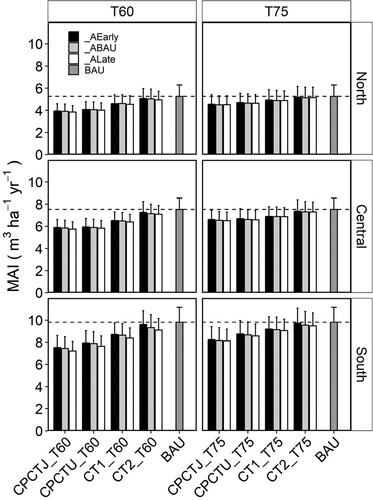
Figure 6. Land expectation value at the time of establishment for different conversion strategies and for the abandonment options AEarly (black), ALate (white) and ABAU (grey). The dashed lines represent LEV of a traditional clear-cutting system (BAU). LEV was calculated as a mean for stands located in northern, central and southern Sweden, using interest rates of 1%, 2% and 3%. For abbreviations of strategies and scenarios, see Figure 2.

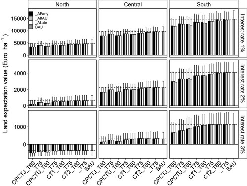
Table 3. Volume of pulpwood and timber and quadratic mean diameter (D_g) at harvest in abandonment option ABAU in relation to a clear-felling system (BAU, 100%) at simulations using 2% interest rate. Separate figures are presented for final felling and for the total removal from the start of the simulation until final felling. For abbreviations of conversion scenarios, see Figure 2.

			Final felling			Total
Strategy	Removal	Aband. timing	Dg	Pulpwood	Timber	Dg	Pulpwood	Timber
CPCTJ	_T60	_ABAU	93	47	43	93	94	70
CPCTU			94	47	44	94	95	74
CT1			91	50	47	96	102	83
CT2			92	53	51	99	99	94
CPCTJ	_T75	_ABAU	94	65	57	97	98	81
CPCTU			94	65	60	98	99	86
CT1			93	65	59	99	102	90
CT2			94	68	64	100	99	97

Skogsstyrelsen. 1985a. Gallringsmallar – södra Sverige. Skogsstyrelsen, Jönköping, Sweden. 35 p. (In Swedish).

 Google Scholar

Skogsstyrelsen. 1989. Gallringsmallar – norra Sverige. [Thinning guidelines – Northern Sweden] Skogsstyrelsen, Jönköping, Sweden. 35 p. (In Swedish).

 Google Scholar

Data availability

Data are available upon request from the corresponding author.