A new method to assess pulmonary changes using ¹⁸F-fluoro-2-deoxyglucose positron emission tomography for lung cancer patients following radiotherapy

Figures & data

Figure 1. Visualizing axial (a) CT and (b) ¹⁸F-FDG-PET images. Left: RT dose distribution registered with planning CT for one patient with dose ranges from 0 to 30 Gy (left most color bars). Right: Δμ, Δσ and ΔS maps were displayed during (top) and six weeks post (bottom) treatment. Units are HU for CT, while PET values are unitless. ΔS maps both in mid- and post-therapy visualized new regions of interest that were not visible in the Δμ maps.

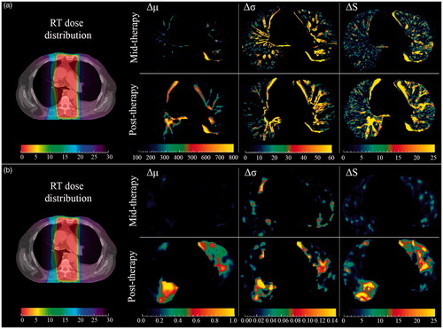
Figure 2. Population based Δμ, Δσ and ΔS dose–response curves based on (a) density (CT-based HU) and (b) ¹⁸F-FDG uptake in the lung at mid- and post-therapy across patients treated with RT. Horizontal gray bars show the mean of changes over entire lung in the control group (mean ± SD).

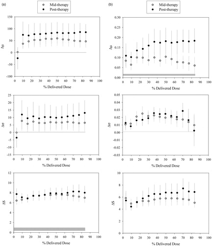
Table 1. Analyses of dose–response relationships.

	Δμ (95% CI)	Δσ (95% CI)	ΔS (95% CI)
CT
Mid-pre
Slope	3.4 (−1.0, 7.7)	0.3 (−0.6, 1.1)	0.1 (−0.1, 0.2)
Intercept	19.5 (−19.8, 58.9)	3.7 (−4.2, 11.6)	6.4 (5.1, 7.7)
Post-pre
Slope	4.9 (−2.5, 12.2)	0.5 (−0.8, 1.8)	0.1 (−0.1, 0.2)
Intercept	26.5 (−41.1, 94.2)	4.4 (−7.6, 16.5)	7.1 (5.7, 8.6)
PET
Mid-pre
Slope	0.1 (−0.3, 0.6)^a	0.1 (0.0, 0.2)^a	0.1 (−0.1, 0.2)
Intercept	7.9 (3.9, 12.0)^a	1.2 (0.3, 2.4)^a	5.2 (3.9, 6.5)
Post-pre
Slope	0.6 (−0.3, 1.5)^a	0.1 (0.0, 0.2)^a	0.2 (0.1, 0.4)
Intercept	0.1 (0.0, 0.2)	0.9 (−0.2, 2.0)^a	4.7 (2.8, 6.6)

Population-based analyses for changes in the pulmonary dose–response parameters between mid-pre and post-pre imaging sessions using either CT or ¹⁸F-FDG-PET scans. Slopes and intercepts with corresponding 95% confidence intervals (CIs) are given.

^a Multiplied by a factor 100.