Influence of gray level discretization on radiomic feature stability for different CT scanners, tube currents and slice thicknesses: a comprehensive phantom study

Figures & data

Table 1. Overview scanners and per scanner exposure time, convolution kernel, tube current, focal spot size and collimation.

Hospital	Vendor	Model	Coding	Exposure time (ms)	Convolution kernel	Tube Current (mA)	Focal spot size (mm)	Collimation (# * mm)
1	Siemens	SOMATOM Definition Flash	Fl	500	B31f	128, 160, 296, 592	1.2	64 * 0.6
	Philips	Brilliance 64	P	561	B	61, 91, 119, 148, 274	1.0	64 * 0.6
2	Siemens	Biograph 40	B	500	B31f	40, 60, 80	1.2	24 * 1.2
	Siemens	SOMATOM Confidence RT Pro	C	1000	B31s	26, 39, 52, 66, 121	1.2	32 * 0.6
	Siemens	SOMATOM Sensation Open	O	500	B31f	60, 80, 100	1.2	24 * 1.2
3	Siemens	SOMATOM Definition Flash	L	500	B31f	64, 96, 128, 162, 296, 594	1.2	64 * 0.6
4	Siemens	SOMATOM Definition AS+	V	500	B31f	64, 96, 128, 162, 298, 594	1.2	64 * 0.6
5	Siemens	Biograph 16	H	500	B31f	40, 60, 84, 112, 140, 216, 274	0.7	16 * 0.75
6	Philips	Gemini TF 16	S	534	B	58, 88, 114, 143, 266, 497	1.0	16 * 1.5

Figure 1. Scatterplots of feature values for all scanners. Per scanner, the data is sorted from high to low exposure. Left: original data; Right: after resampling; Top: ‘GLRLM–RLN’, highest slice thickness dependency; Bottom: ‘GLSZM – SAE’, lowest slice thickness dependency.

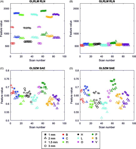
Figure 2. Bar plots of the spread of feature values of (A): ‘GLRLM–RLN’ and (B): ‘GLSZM – SAE’. Bars range from the minimum to the maximum observed value, and the vertical lines indicate the median. From top to bottom these bars are shown for all scans (n = 90), all scans with an exposure of 60 mA (n = 6), all scans with an exposure of 80 mA (n = 4), all scans with an increment of 1 mm (n = 34), 2 mm (n = 34) and 3 mm (n = 13) and all scans after resampling the images into 1 × 1 × 3 mm³ using cubic (n = 90), linear (n = 90) and nearest neighbor (n = 90) interpolation.

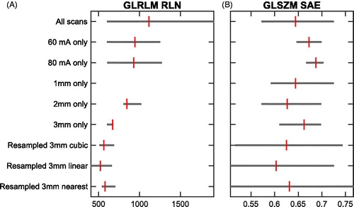
Figure 3. HU distributions of the rubber insert scanned with a fixed CDTI of 5.43 mGy on five different Siemens and Philips scanners. From left to right and top to bottom [scanner - tube current]: ‘Fl-160mA’, ‘L-161mA’, ‘P-148mA’, ‘S-143mA’, and ‘V-162mA’. The scatterplot in the bottom right displays the observed values of the feature ‘GLCM cluster prominence’ over all scanners. The outlier in dark-green is scanner ‘P’.

Figure 4. Normalized feature values plotted against bin width. (A): GLCM features (n = 26), (B): GLDZM features (n = 16), (C): GLRLM features (n = 16), (D): GLSZM features (n = 16), (E): NGDLM features (n = 16), (F): NGTDM (n = 5) and first order statistics features (n = 2, dotted lines). The red dashed lines indicate GLRLM RLN and GLSZM SAE.

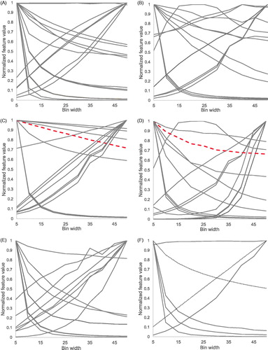
Figure 5. The total number of features with a CCC > 0.85 for each bin width when comparing (A) a slice thickness of 1.5 mm with 3 mm (exposure 60 mA, scanner ‘B’), (B) an exposure of 60 mA with 80 mA (slice thickness 3 mm, scanner ‘B’), or (C) scanner ‘B’ with ‘O’ using the same scan protocol (exposure 60 mA and slice thickness 3 mm). Test-retest figures are based on the minimal observed CCC in both test-retest sets that are compared.

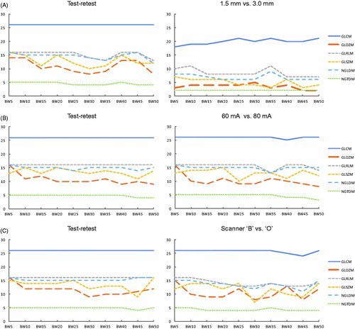
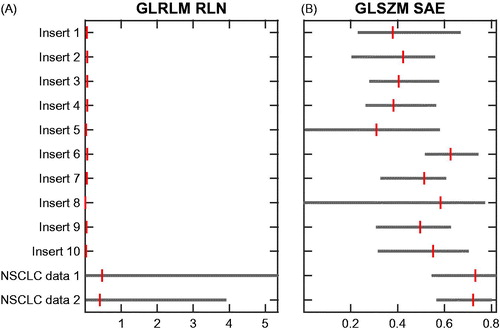
Figure 6. Bar plots of the spread of feature values over all phantom inserts and two independent NSCLC datasets for (A): ‘GLRLM – RLN’ and (B): ‘GLSZM–SAE’. The bars indicate the minimum, median and maximum feature values. Scans were resampled to 1 × 1 × 3 mm³ voxels using cubic interpolation and a bin width of 25 HU was used.