Tumor volume regression during preoperative chemoradiotherapy for rectal cancer: a prospective observational study with weekly MRI

Figures & data

Table 1. Patients characteristics.

Gender (n)
Male	14
Female	1
Age (mean ± SD; range)	60 ± 8; 38–73
Clinical stage before treatment (n)
cT2 N2	1
cT3 N0–2	13
cT4 N2	1
Pathological stage (n)
ypT0 N0 (pCR)	3
ycT0 N0 (ypTx Nx)	1
ypT1–2 N0–1	6
ypT3 N0–2	5
Initial tumor volume (cc) (mean ± SD; range)	53.6 ± 32.8; 16–138
Total treatment time (days) (mean ± SD; range)	34.4 ± 1.8; 31–37

SD: standard deviation.

Figure 1. Example of tumor regression over time in a single patient (sagittal T₂-weighted images). Decrease in GTV volume (red) is already visible in the first week of CRT.

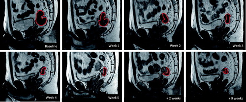
Figure 2. Evolution of target volumes (mean ± standard deviation) over time, relative to baseline volume, for GTV (red) and PTV (blue). N = 15. Asterisk (*) denotes significant difference with previous time-point (p < .007). Other p values range between .01 and .07.

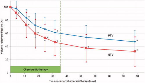
Table 2. Mean tumor volumes at different time points during and after therapy (n = 15).

	Before CRT	Week 1	Week 2	Week 3	Week 4	Week 5	2–4 weeks after CRT	7–8 weeks after CRT
Mean overall treatment time (days)	0	3.9	10.9	17.1	23.9	31.1	54.0	88.1
GTV volume (cc)	53.6	49.0*	40.0*	31.8*	28.7*	25.1*	20.6*	17.7*
GTV volume relative to baseline (%)	100	91.5	73.1	59.7	53.2	46.3	37.3	32.4
PTV volume (cc)	166.7	158.6	135.6*	116.3	105.1	97.7*	87.2	76.7*
PTV volume relative to baseline (%)	100	97.9	83.7	72.1	66.5	61.2	53.9	47.2

*p < .007, difference compared to previous measurement.

Figure 3. Speed of GTV shrinkage over the CRT course (mean ± standard deviation). (A) Absolute shrinkage per week (expressed in % relative to the baseline volume). (B) Shrinkage relative to the previous measurement (%/week). (N = 15; Post 1 and 2: respectively 2–4 weeks and 7–8 weeks post CRT).

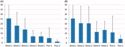
Table 3. Average PTV boost volume reduction using different adaptive strategies.

Adaptive strategy	Optimal adaptation at fraction	Average reduction in treated volume (%)
None	–	0
SIB: 1 adaptation	13	12.4
SIB: 2 adaptations	12;17	15.5
SIB: 3 adaptations	8;12;17	17.0
SIB: 4 adaptations	8;12;17;22	17.9
SIB: 5 adaptations	7;9;12;17;22	18.3
SIB: 24 adaptations (next fraction)	Daily	20.0
SIB: 25 adaptations (same fraction)	Daily	21.6
Sequential boost	After first course	39

Treated volume is the average PTV boost over the treatment course, relative to baseline PTV. Optimal time points are calculated assuming planning imaging was done the fraction before.