Proton range shift analysis on brain pseudo-CT generated from T1 and T2 MR

Figures & data

Figure 1. The lower part of the head was cropped because of the noise that would have altered the automatic segmentation process. After that, a foreground masking and a registration of the three modalities were performed in order to increase the accuracy of the pCT generation algorithm.

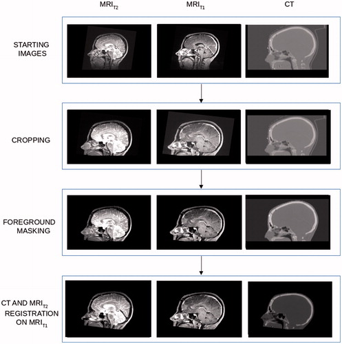
Figure 2. Average HU value calculation: for each 10 × 10 T1_w/T2_w intensity bin, the average value is calculated, thus returning the HU value on the pCT for that patch.

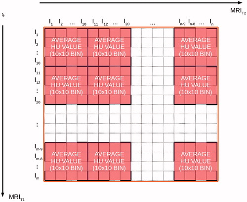
Figure 3. Visual comparison between pCT (a and c) and CT (b and d) for two representative cases. The zygomatic and frontal bones and the sinus cavities are most affected by wrong HU reassignment (c and d). The surgical holes present in the posterior left region of the skull (a and b) are satisfactorily reconstructed.

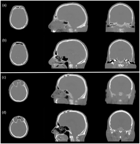
Figure 4. The dose profile is evaluated on a central line along the slices of the dose volume (a). For the same slice it the dose distribution and HU values for both pCT and CT along the beam line are plotted (b).

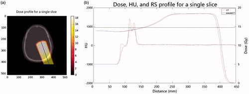
Figure 5. Frequency distribution of the signed RS for all patients, in which the normal distribution of the RS can be observed. Example of dose profile with R₈₀ for pCT and CT, and the relative RS.

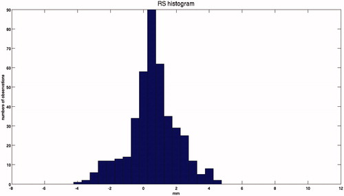
Figure 6. DVH of the total dose delivered to the PTV and OAR (consisting of a 2-cm region surrounding the outside of the PTV) for patients 1, 2, 11 and 14. Blue lines are for pCT and red for CT.

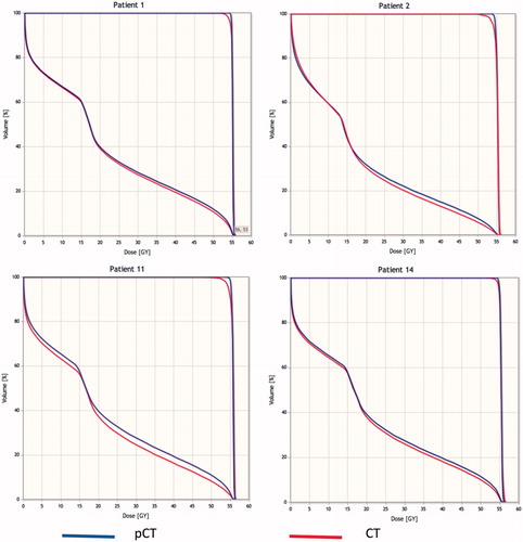
Table 1. Relative range shift, range shift test and γ-index test for each patient.

												RS test
						Relative range shift								γ–index test
Patient	Beam	Slice 01	Slice 02	Slice 03	Slice 04	Slice 05	Slice 06	Slice 07	Slice 08	Slice 09	Slice 10	MGH	HTPI	2%/2 mm
	AX1	0.40	0.46	0.53	0.32	0.27	0.52	0.47	0.55	0.25	0.18	√	√
1	AX2	0.95	0.60	0.54	0.91	0.49	0.69	0.80	0.69	0.51	0.40	√	√	96.97
	CC	5.71	6.30	7.16	6.79	6.30	5.71	7.61	8.90	7.49	5.64	x	x
	AX1	6.11	4.86	4.93	5.17	5.21	6.14	6.40	5.49	3.38	1.81	√	√
2	AX2	2.75	1.78	1.30	1.30	1.84	2.19	1.23	1.27	1.03	1.67	√	√	94.09
	CC	2.13	2.17	1.88	2.04	1.95	1.97	2.06	2.28	2.22	2.34	√	√
	AX1	2.66	2.18	1.98	1.60	2.32	2.24	2.30	2.80	2.80	2.89	√	√
3	AX2	3.15	2.97	3.00	2.98	3.04	2.81	2.72	2.69	2.80	2.88	√	√	99.39
	CC	1.09	1.44	0.98	1.04	0.95	0.77	0.88	1.09	1.11	0.72	√	√
	AX1	1.63	1.98	1.96	2.03	2.04	2.36	3.37	4.59	3.46	3.80	√	√
4	AX2	−0.66	−0.68	−0.61	−0.62	−0.57	−0.62	−0.96	−1.77	−2.27	−2.37	√	√	99.81
	CC	0.72	−0.67	−1.44	−2.73	−3.80	−5.54	−5.93	−4.75	−1.85	−0.30	√	√
	AX1	−0.35	−0.76	−0.71	−1.02	−0.95	−1.00	−1.18	−1.47	−1.42	−1.20	√	√
5	AX2	2.28	0.63	−2.92	−2.81	−1.42	−1.21	−0.19	0.11	0.23	0.24	√	√	99.11
	CC	3.56	3.67	3.88	4.04	4.07	4.02	3.64	2.48	1.04	0.73	√	√
	AX1	−0.19	0.04	0.31	0.36	0.37	0.41	0.41	0.60	0.49	1.37	√	√
6	AX2	0.69	0.73	0.71	0.81	0.91	0.83	0.69	0.57	0.65	0.77	√	√	100
	CC	0.03	0.29	0.36	0.28	0.15	0.10	0.05	0.01	0.00	0.07	√	√
	AX1	1.67	1.60	1.56	1.41	1.35	1.62	1.63	1.34	1.51	1.23	√	√
7	AX2	−0.03	−0.43	−0.93	−0.99	−1.16	−0.73	−0.66	−0.40	−0.63	−0.94	√	√	99.98
	CC	0.18	0.27	0.33	0.27	0.30	0.38	0.55	0.57	0.43	0.35	√	√
	AX1	1.36	1.24	1.23	1.20	1.29	1.29	1.09	1.57	1.07	1.96	√	√
8	AX2	1.06	0.66	0.63	0.77	0.75	0.75	0.97	1.19	1.12	0.98	√	√	100
	CC	1.44	0.54	−0.61	−0.62	0.04	0.83	1.17	1.74	2.75	2.97	√	√
	AX1	−0.69	−0.78	−0.46	−0.42	−0.52	−0.54	−0.50	−0.42	−0.30	−0.21	√	√
9	AX2	1.53	1.42	1.22	1.26	1.44	1.41	1.39	1.48	1.35	1.53	√	√	100
	CC	0.12	0.28	0.23	0.32	0.61	0.78	0.45	0.18	−0.10	−0.34	√	√
	AX1	1.04	2.51	0.88	0.80	0.58	0.90	0.55	0.48	0.64	0.49	√	√
10	AX2	0.74	0.60	0.97	1.11	1.21	0.84	0.83	2.24	1.89	1.52	√	√	100
	CC	−1.81	−1.83	−1.98	−1.52	−1.74	−1.92	−2.00	−2.14	−2.16	−1.55	√	√
	AX1	2.13	3.32	3.96	3.94	4.38	3.57	3.75	4.14	3.99	4.25	√	√
11	AX2	3.26	2.59	1.97	2.61	1.62	1.73	1.83	1.76	1.73	1.82	√	√	96.61
	CC	3.48	3.29	3.24	3.27	3.33	3.34	3.82	3.85	4.12	3.98	√	√
	AX1	−2.37	−2.36	−2.34	−2.17	−2.44	−2.39	−2.20	−2.36	−2.63	−2.49	√	√
12	AX2	−0.25	−0.32	−0.16	−0.08	−0.04	0.00	−0.04	−0.26	−0.64	−1.02	√	√	100
	CC	0.51	0.54	0.49	0.42	0.52	0.82	0.83	1.03	0.93	0.98	√	√
	AX1	−5.95	−2.33	−2.05	−2.21	−5.25	−2.27	−2.44	−3.37	−3.55	−3.20	√	√
13	AX2	1.16	1.05	0.60	0.58	0.72	0.77	1.05	1.00	2.08	0.82	√	√	100
	CC	−4.12	−4.33	−4.18	−0.94	−3.83	−3.78	−3.97	−4.38	−4.24	−4.28	√	√
	AX1	2.67	2.46	2.71	3.18	3.29	3.27	3.15	3.05	3.52	4.75	√	√
14	AX2	1.42	1.65	4.95	1.13	1.13	1.45	1.88	2.32	1.56	5.77	√	√	99.64
	CC	7.84	8.01	9.42	10.5	6.42	−0.25	−2.88	−1.16	0.41	3.27	x	x

Italic and bold cells represent presence, along the beam, of air and metal, respectively.

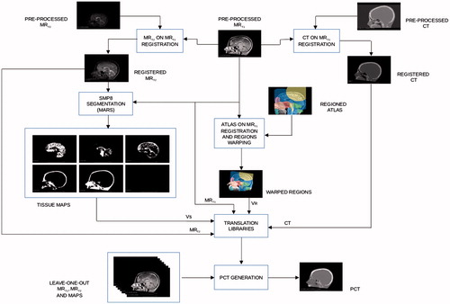
Figure 7. Flow chart for the generation of the conversion libraries.