Pharmacokinetic analysis of DCE-MRI data of locally advanced cervical carcinoma with the Brix model

Figures & data

Table 1. Patient characteristics (N = 80).

Characteristic
Age, years
Median	57
Range	22 − 88
Histology, #patients
Squamous cell carcinoma	68
Adenocarcinoma	10
Undifferentiated	2
Volume, cm^3
Median	40.7
Range	2.1 − 319
FIGO stage, #patients
I	7
II	55
III	15
IV	3
Pelvic lymph node status, #patients
Positive	35
Negative	45

Figure 1. A_Brix, k_ep, and k_el frequency distributions, parametric images, and binary images highlighting RV-A_Brix, RV-k_ep, and RV-k_el in dark gray for a representative high-enhancing (a) and a representative low-enhancing (b) tumor. The frequency distributions include all tumor voxels, whereas the images refer to a single slice through the tumor. To avoid presenting the entire tail of the frequency distributions, the last column of the distributions represents the percentage of voxels with A_Brix ≥ 3.0, k_ep ≥ 10, and k_el ≥ 0.15. The vertical lines in the frequency distributions represent the threshold A_Brix, k_ep, and k_el values of RV-A_Brix, RV-k_ep, and RV-k_el (solid lines) and the median values of A_Brix, k_ep, and k_el (dashed lines). Scale bars: 1 cm.

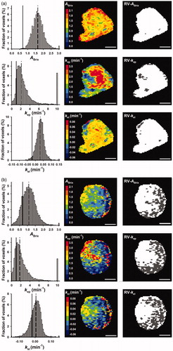
Figure 2. The tumor volumes with voxel values below a threshold value were calculated from the A_Brix, k_ep, and k_el frequency distributions of all tumors, using a range of threshold values for each parameter, and for each threshold value, the outcome of the patients with large volumes were compared with that of the patients with small volumes, using the log-rank test with DFS and OS as endpoints. ROC analysis was carried out to find the threshold values with the highest discriminative power. The plots show the log-rank p-value (a) and the area under the ROC-curve (b) versus A_Brix, k_ep, and k_el threshold value for DFS and OS. The dashed lines in (a) represent a significance level of p = .05. The vertical lines in (b) represent the optimal threshold values for A_Brix, k_ep, and k_el.

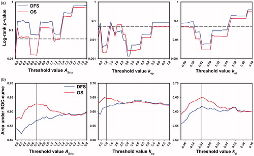
Figure 3. Kaplan–Meier curves for DFS and OS stratified by RV-A_Brix (a), RV-k_ep (b), and RV-k_el (c). The cutoffs separating small (N = 54) from large (N = 26) RVs were 1.3 cm³ for RV-A_Brix, 0.9 cm³ for RV-k_ep, and 1.1 cm³ for RV-k_el.

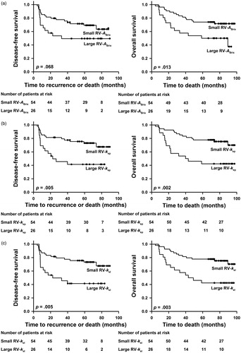
Table 2. Cox regression analysis of clinical and Brix parameters.

	Univariate		Multivariate
	Disease-free survival	Overall survival	Disease–free survival			Overall survival
	p-value	p-value	p-values^a			p-values^a
Tumor volume	.026	.019	.89	.99	.77	.77	.60	.92
FIGO stage	.0057	.017	.052	.060	.043	.065	.10	.061
Lymph node status	.13	.36	.73	.72	.78	.82	.76	.63
Tumor histology	.30	.31	–	–	–	–	–	–
Patient age	.30	.17	–	–	–	–	–	–
RV-ABrix	.015	.00058	.16	–	–	.018	–	–
RV-kep	.00060	.000060	–	.020	–	–	.0033	–
RV-kel	.0011	.000056	–	–	.030	–	–	.0030

Values of p < .05 are highlighted in bold.

^ap-values refer to multivariate regression analyses including tumor volume, FIGO stage, lymph node status, and either RV-A_Brix, RV-k_ep, or RV-k_el.

RV-A_Brix, tumor volume with A_Brix < 0.7; RV-k_ep, tumor volume with k_ep < 1.0; RV-k_el, tumor volume with k_el < −0.02.

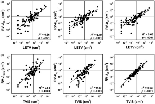
Figure 4. Log scale plots of RV-A_Brix, RV-k_ep, and RV-k_el versus LETV (a) and TVIS (b). Six tumors had LETV of zero, and to be able to include these tumors in the log scale plots, they were assigned LETV corresponding to one voxel. The patient cohort was divided into two groups consisting of one third and two-thirds of the patients, and the discrimination levels are indicated by horizontal lines for RV-A_Brix, RV-k_ep, and RV-k_el and by vertical lines for LETV and TVIS. Points refer to individual tumors. Curves were fitted to the points by linear regression analysis.