Impact of NaOH based perfusion-decellularization protocol on mechanical resistance of structural bone allografts

Figures & data

Figure 1. Cutting steps. A: Decellularized and control pair. Dots on bones show section planes. Decellularized samples are shown with an asterisk. B: Band saw cutting. C: Polishing phase. D: Final samples for each test, S + I = Screw pull-out + Indent; B = 3-points bending; T= torsion; C= Compression.

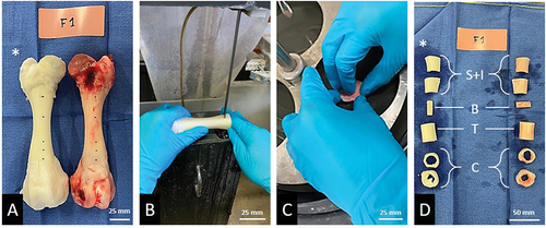
Figure 2. Screw pull-out test. A: Sample drilling with a 3D-printed guide. The asterisk shows the tested bone sample. B: Image of a 3.5 mm cortical screw inserted in the sample. C: Installation. The arrow shows the head of the screw sliding into the dedicated clamp. D: During the test, the bone is fixed by nuts. The arrow shows the rupture of the bone.

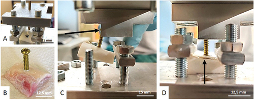
Figure 3. Three points bending test. A: Pre-loading image of the sample marked by an asterisk. B: Loading of the sample before fracture. C: Extrapolation of the model for the mathematical results. 1 = actual dimension of the sample, 2 = the rectangular volume chosen for the mathematical operation.

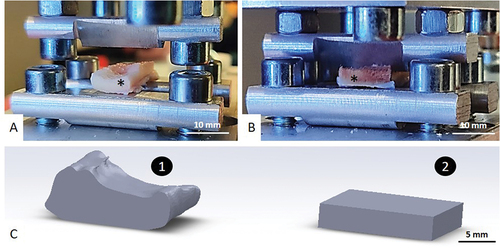
Figure 4. Torsion test. A: Designing and prototyping of the custom-made torsiometer. 1=sample; 2=distributor; 3= point of transformation from a rotative movement to a linear movement; 4= weights holder; 5 = 100 g load; 6= screws area. B: Centering and fixation of the sample. The black asterisks show the bone samples. C: inside the torsiometer, black arrows show the fixed side of the element, blue arrows show the rotating side of the element. D: Complete set-up during experiment. Red asterisks show the distributor and red arrow shows the infra-millimetric gauge measuring displacement at the very end of the lever arm.

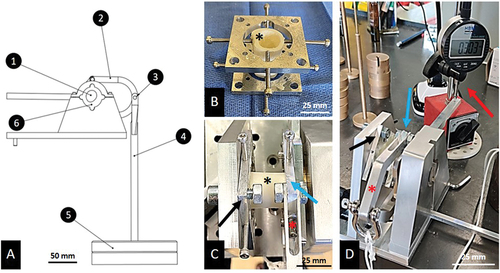
Figure 5. Compression test. A: Pre-loading sample. B: Loaded sample after fracture occurrence. Subtle fracture lines are pointed out by white arrows. C: Transversal CT-scan acquisition of post-compression test showing fracture lines (white arrows). D: Axial CT-scan acquisition of post-compression test showing fracture lines (white arrows).

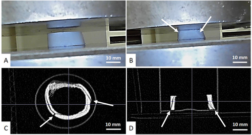
Figure 6. Vickers hardness test. A: Medullary view of a sample after screw pull-out. Red rectangles show the cut plane where the indent will be performed. White asterisk shows the screw mark. B: Embedded samples exposing the cut plane. C: microscopic view of a punch on a bone surface.

Figure 7. Boxplots of the 12 measured variables during the 5 mechanical tests. S: boxplots from the screw pull-out test. B: boxplots from the 3-points bending test. T: boxplot from the torsion test. C: boxplots from the compression test. I: boxplot from the indentation/Vickers test. * = Lightly significant; ns = not significant.

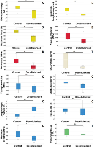
Table 1. Descriptive statistics of the variables from the screw pull-out test.

Variable	Treatment	Mean	Standard deviation	95% IC	Variance	Range
Maximum force (N)	Control	602.31	128.21	443.11–761.50	16437.72	330.06
	Decellularized	419.76	110.23	282.90–556.63	12150.09	235.64
Maximum Lengthening (mm)	Control	1.25	0.27	0.92–1.59	0.07	0.73
	Decellularized	0.90	0.20	0.65–1.15	0.04	0.55
Extraction energy (J)	Control	0.31	0.07	0.23–0.39	0.01	0.19
	Decellularized	0.21	0.07	0.12–0.30	0.01	0.14

Table 2. Descriptive statistics of the variables from the 3-points bending test.

Variable	Treatment	Mean	Standard deviation	95% IC	Variance	Range
Young’s modulus (MPa)	Control	1281.57	603.07	532.76–2030.39	363697.40	1435.90
	Decellularized	724.96	632.08	−59.86–1509.79	399520.45	1575.61
Resistance (MPa)	Control	194.52	67.08	111.22–277.82	4500.46	160.11
	Decellularized	98.11	42.37	45.5–150.72	1795.25	107.29

Table 3. Descriptive statistics of the Shear’s modulus from the torsion test.

Variable	Treatment	Mean	Standard deviation	95% IC	Variance	Range
Shear’s modulus (MPa)	Control	339.56	71.58	225.67–453.46	5123.21	135.24
	Decellularized	280.95	11.46	262.71–299.19	131.40	25.30

Table 4. Descriptive statistics of the variables from the compression test.

Variable	Treatment	Mean	Standard deviation	95% IC	Variance	Range
Young’s modulus (MPa)	Control	1028.46	163.55	825.39–1231.54	26746.19	429.80
	Decellularized	916.40	109.25	780.74–1052.05	11936.50	245.94
Elastic limit (MPa)	Control	22.60	3.67	18.04–27.16	13.49	10.32
	Decellularized	19.79	2.81	16.30–23.28	7.92	6.81
Maximum constrain (MPa)	Control	92.60	28.53	57.18–128.03	813.95	74.13
	Decellularized	63.87	15.31	44.85–82.88	234.42	35.98
Maximum lengthening (mm)	Control	3.75	4.11	−1.35–8.85	16.86	10.39
	Decellularized	8.06	4.72	2.20–13.92	22.29	12.92
Resilience (J)	Control	6.21	0.50	5.59–6.82	0.25	1.34
	Decellularized	6.10	0.85	5.04–7.16	0.73	2.11

Table 5. Descriptive statistics of the Hardness Value from the Indentation/Vickers test.

Variable	Treatment	Mean	Standard deviation	95% IC	Variance	Range
Hardness Value (HV)	Control	38.82	4.72	32.96–44.68	22.27	10.81
	Decellularized	36.68	7.24	27.68–45.67	52.48	20.48