Figures & data
Figure 1. In each recruitment cycle, new users of drug A and new users of drug B are included and added to the cohort to continuously increase the study sample size.
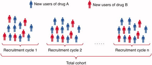
Figure 2. Effect estimates are published after each recruitment cycle.
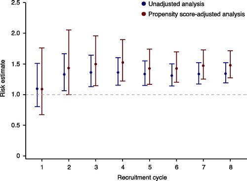
Figure 3. Standardized differences in baseline covariates between new users of drug A and new users of drug B before and after adjusting on the propensity score. A standardized difference <0.1 indicates negligible imbalance.
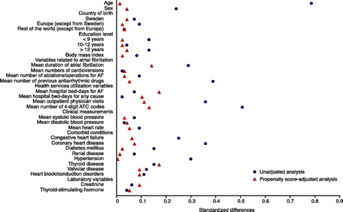
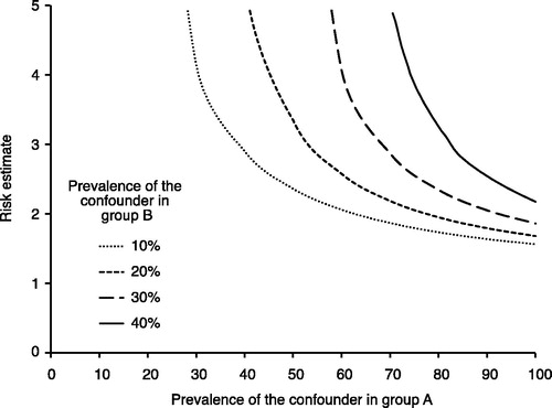
Figure 4. Evaluation of how powerful an unmeasured confounder would have to be to change the observed results. For example, if the prevalence of a potential unmeasured confounder is 40% in the drug A group (x-axis) and 10% in the drug B group, then the unmeasured confounder must have a risk estimate (hazard ratio) of the outcome close to 3 to fully explain the advantage of drug A over drug B.