2,352
Views
2
CrossRef citations to date
0
Altmetric
Original Articles

A splitting algorithm for simulation-based optimization problems with categorical variables

ORCID Icon, ORCID Icon, ORCID Icon, ORCID Icon & ORCID Icon
Pages 815-831 | Received 30 May 2017, Accepted 09 Jun 2018, Published online: 30 Jul 2018

Figures & data

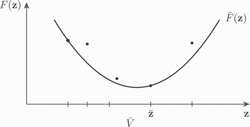
Figure 1. Illustration of the quadratic underestimating function F¯. The objective function F is evaluated at the set of sample points V¯ (illustrated by the dots).

Figure 1. Illustration of the quadratic underestimating function F¯. The objective function F is evaluated at the set of sample points V¯ (illustrated by the dots).

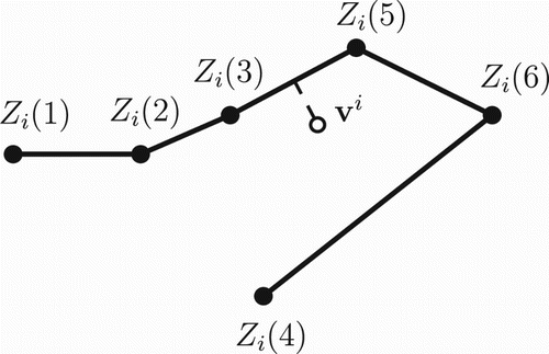
Figure 2. Illustration in R2 of the nearest edge projection splitting strategy. The split is identified across the edge Zi(3)Zi(5) of the minimum spanning tree corresponding to the designs Zi(Xis)={Zi(1),,Zi(6)} by projecting (illustrated by the dashed line) the solution to (Equation3), in terms of vi, onto the tree.

Figure 2. Illustration in R2 of the nearest edge projection splitting strategy. The split is identified across the edge Zi(3)–Zi(5) of the minimum spanning tree corresponding to the designs Zi(Xis)={Zi(1),…,Zi(6)} by projecting (illustrated by the dashed line) the solution to (Equation3(3a) minimizev,λF¯(v1,…,vm),(3a) ), in terms of vi, onto the tree.

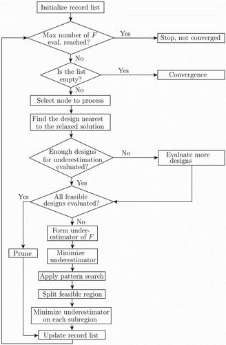
Figure 3. Flowchart of the algorithm quadDS.

Figure 3. Flowchart of the algorithm quadDS.

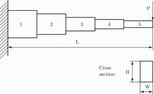
Figure 4. A stepped cantilever beam with m=5 segments.

Figure 4. A stepped cantilever beam with m=5 segments.

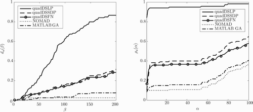
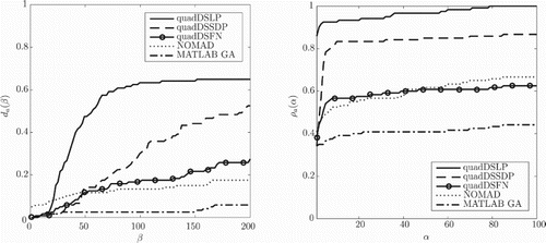
Figure 5. Data profiles da(β) and performance profiles ρa(α) for three variants of quadDS, the MATLAB GA and NOMAD applied to 120 instances of the sparse artificial problem with τ=0.1.

Figure 5. Data profiles da(β) and performance profiles ρa(α) for three variants of quadDS, the MATLAB GA and NOMAD applied to 120 instances of the sparse artificial problem with τ=0.1.

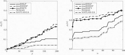
Figure 6. Data profiles da(β) and performance profiles ρa(α) for three variants of quadDS, the MATLAB GA and NOMAD applied to 120 instances of the fully artificial problem with τ=0.1.

Figure 6. Data profiles da(β) and performance profiles ρa(α) for three variants of quadDS, the MATLAB GA and NOMAD applied to 120 instances of the fully artificial problem with τ=0.1.

Figure 7. Data profiles da(β) and performance profiles ρa(α) for three variants of quadDS, the MATLAB GA and NOMAD applied to 120 instances of the beam problem with τ=0.1.

Figure 7. Data profiles da(β) and performance profiles ρa(α) for three variants of quadDS, the MATLAB GA and NOMAD applied to 120 instances of the beam problem with τ=0.1.

Figure 8. Data profiles da(β) and performance profiles ρa(α) for three variants of quadDS, the MATLAB GA and NOMAD applied to 120 instances of the tyres selection problem with τ=0.001. Note that dNOMAD(β)=0 for all values of β and ρNOMAD(α)=0.5 for all values of α, because NOMAD did not solve any of the instances of the tyres selection problem within the maximum allowed number of objective function evaluations.
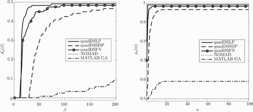
Figure 8. Data profiles da(β) and performance profiles ρa(α) for three variants of quadDS, the MATLAB GA and NOMAD applied to 120 instances of the tyres selection problem with τ=0.001. Note that dNOMAD(β)=0 for all values of β and ρNOMAD(α)=0.5 for all values of α, because NOMAD did not solve any of the instances of the tyres selection problem within the maximum allowed number of objective function evaluations.