Rescaling the land rush? Global political ecologies of land use and cover change in key scenario archetypes for achieving the 1.5 °C Paris agreement target

Figures & data

Figure 1. Google scholar results (‘political ecology’ AND ‘ … ’). Data: Google scholar (29 July 2021).

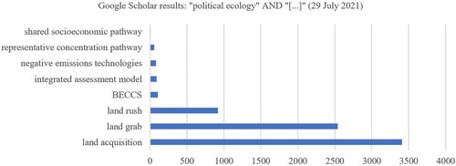
Figure 2. Rural population across global south and global north according to different population projections. 1960–2018 historical data (FAO). 2060–2100 projection (IIASA). SSP5 data not included, given a strong similarity with SSP1. SSP2 data not included, as it is identical with LED. SSP1 is based on IMAGE model, LED is based on MESSAGEix-GLOBIOM model.

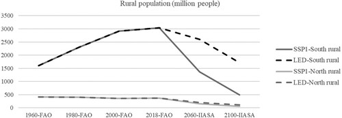
Table 1. Future population and urbanization dynamics and underlying assumptions. (Based on Jiang and O’Neill 2017; Riahi et al. 2017; Grubler et al. 2018). Data for urbanization rate: Jiang and O’Neill 2017. Population data: FAO-historical, IIASA-projected.

	SSP1 and SSP5	SSP2 and LED
Global population, first half of twenty-first century	Moderate population growth	High population growth
Global population, second half of twenty-first century	High overshoot (at 8.5 billion) and shrinking population (to 7 billion)	Low overshoot (9.5 billion) and stabilization at 9 billion
Global population, 2010 vs 2100	Almost identical (around 7 billion)	Growth from 7 to 9 billion
Urbanization rate (World)	High urbanization rate (from 60% in 2020 to 92% in 2100)	Moderate urbanization rate (from 56% in 2020 to 79% in 2100)
Urbanization rate (Global South)	High (from 49/84/53% in 2020 to 90/95/91% in 2100 –Africa/Latin America/Asia)	Moderate (from 46/82/48% in 2020–73/91/78% in 2100 –Africa/Latin America/Asia)
Modelled assumptions	Increased migration and fast urbanization due to medium to high economic growth, high income growth, relatively low income inequality, ‘environmentally friendly living arrangements’ (SSP1); high economic growth and technological change, increasing agricultural productivity, growing wealth (SSP5)	Moderate income and economic growth, and moderate socio-economic inequality lead to moderate urbanization rate, in line with historical development. LED scenario with much more aggressive assumptions concerning reductions in consumption, energy conservation or efficiency, industrial activity, and therefore final global energy demand

Figure 3. World land use/cover change (in millions of hectares in 2100, relative to 2010 reference levels) in key emissions reduction pathways under baseline (no additional mitigation policies) and mitigation policy conditions for limiting global warming to 1.5 °C above pre-industrial averages (RCP1.9). Data: © IAMC 1.5 °C scenario explorer hosted by IIASA https://data.ene.iiasa.ac.at/iamc-1.5c-explorer (see Huppmann et al. 2018).

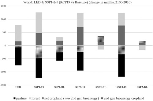
Figure 4. World land use/cover change in absolute (left panel) and relative terms (right panel), in key emissions reduction pathways for limiting global warming to 1.5 °C above pre-industrial averages. Each SSP archetype represents averaged outputs across all available IAMs. LED archetype is based on a single IAM model. Data: © IAMC 1.5 °C scenario explorer hosted by IIASA https://data.ene.iiasa.ac.at/iamc-1.5c-explorer (see Huppmann et al. 2018).

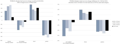
Figure 5. Global north vs Global south - absolute (left panel) and relative (right panel) land use/cover change, in key emissions reduction pathways for limiting global warming to 1.5 °C above pre-industrial averages. Data: © IAMC 1.5 °C scenario explorer hosted by IIASA https://data.ene.iiasa.ac.at/iamc-1.5c-explorer (see Huppmann et al. 2018).

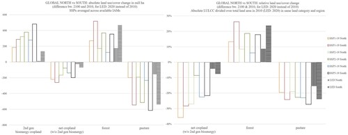
Figure 6. Global south - regional land use/cover change in absolute (left panel) and relative terms (right panel) in key emissions reduction pathways for limiting global warming to 1.5 °C above pre-industrial averages. MAF: Middle East & Africa; LAM: Latin America; ASIA: most Asian countries with exception of Middle East, Japan and former Soviet Union states. Data: © IAMC 1.5 °C scenario explorer hosted by IIASA https://data.ene.iiasa.ac.at/iamc-1.5c-explorer (see Huppmann et al. 2018).

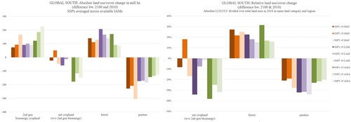
Figure 7. Historical and future land use/cover, globally (in different shades of blue). Historical land use/cover in Global South (black) and Global North (grey). Historical data (1961–2000) from FAO, future data (2010–2100) from IIASA.

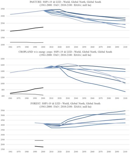
Figure 8. Rate of mean annual net LULCC: Future (LED and SSPx archetypes) and historic (FAO 1961-2000). SSPx = averaged across SSP1, 2, and 5. Data: IIASA/Huppmann et al. (2018), FAO.

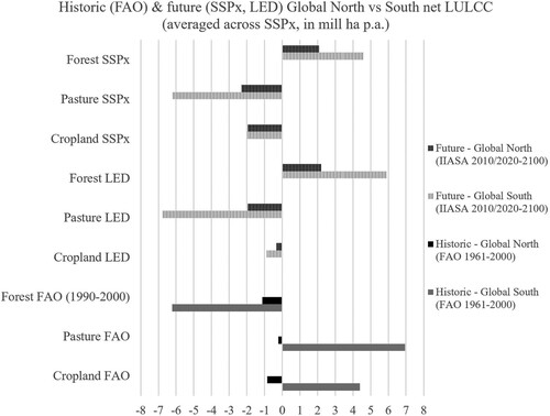
Figure 9. Global North vs Global South - historic and future land availability per rural person (top panel: Cropland, bottom panel: Pasture).

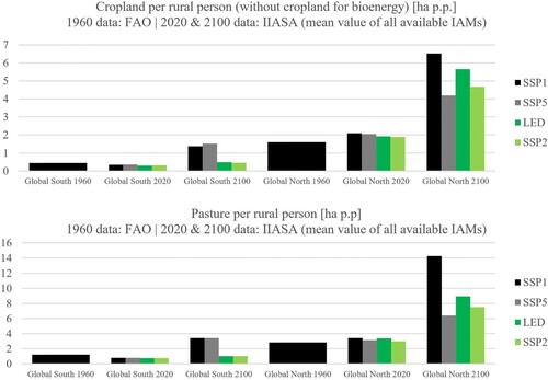
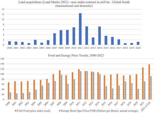
Figure 10. Land acquisitions per year, Global South, 2000–2020 (top panel) and FAO food price index and europe brent spot price (annual average, 2000–2022) (bottom panel). Data: Land Matrix Database, FAO and US EIA (2022).

Jiang, L., and B. C. O’Neill. 2017. “Global Urbanization Projections for the Shared Socioeconomic Pathways.” Global Environmental Change 42: 193–199. doi:10.1016/j.gloenvcha.2015.03.008

 Web of Science ®Google Scholar

Riahi, K., D. P. Van Vuuren, E. Kriegler, J. Edmonds, B. C. O’neill, S. Fujimori, … W. Lutz. 2017. “The Shared Socioeconomic Pathways and Their Energy, Land use, and Greenhouse gas Emissions Implications: An Overview.” Global Environmental Change 42: 153–168. doi:10.1016/j.gloenvcha.2016.05.009

 Web of Science ®Google Scholar

Grubler, A., C. Wilson, N. Bento, B. Boza-Kiss, V. Krey, D. L. McCollum, … J. Cullen. 2018. “A low Energy Demand Scenario for Meeting the 1.5 °C Target and Sustainable Development Goals Without Negative Emission Technologies.” Nature Energy 3 (6): 515–527. doi:10.1038/s41560-018-0172-6

 Web of Science ®Google Scholar

Huppmann, D., E. Kriegler, V. Krey, K. Riahi, J. Rogelj, S. K. Rose, J. Weyant, et al. 2018. IAMC 1.5°C Scenario Explorer and Data Hosted by IIASA. Vienna: Integrated Assessment Modeling Consortium & International Institute for Applied Systems Analysis. doi:10.22022/SR15/08-2018.15429http://doi.org/(accessed 22.10.2020).

 Google Scholar