An ECG simulator with a novel ECG profile for physiological signals

Figures & data

Figure 1. Basic constitution of an ECG segment of physiological type with characteristic waves and spikes [4]. The IBT toolbox [10,11] is capable of detecting 12 characteristic points (P0–P11) from which seven are of interest for this study. POI: Points of interest; Int: Interval; Seg: Segment; Comp: Complex.

Figure 2. Course of heart rate during a stress test ECG. The wide variety of frequencies covered is beneficial for approximating of the temporal ECG profile and therefore of interest for this study.

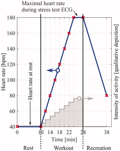
Figure 3. Visual representation of ECG template generation. At the beginning, each individual ECG segment is identified based on its R-peak. Next, the associated heart rate (HR) is determined by inclusion of neighbouring R-peaks according to Equation (1)(1) $$\mathit{HR}\left(i\right)=\frac{60}{\frac{T_{\text{RR}(\mathrm{i}-1)}+T_{\text{RR}\left(\mathrm{i}\right)}}{2}}=\frac{120}{T_{\text{RR}(\mathrm{i}-1)}+T_{\text{RR}\left(\mathrm{i}\right)}}\left[\mathit{bpm}\right]$$(1) . Afterwards, all segments with equal heart rate are organised in the same group and aligned such that R-peaks are congruent. If at least 15 segments are contained in a respective group, ECG templates for that HR are obtained by averaging all segments, which attenuates high-frequency noise.

Figure 4. Heart rates (HR) of an individual during rest and workout. Motion artefacts introduce disturbances into the ECG recording that prevent correct R-peak detection. Thus, the change in HR from one beat to another is compared to the mean heart rate variability (MHRV) to indicate and exclude outliers from further processing.

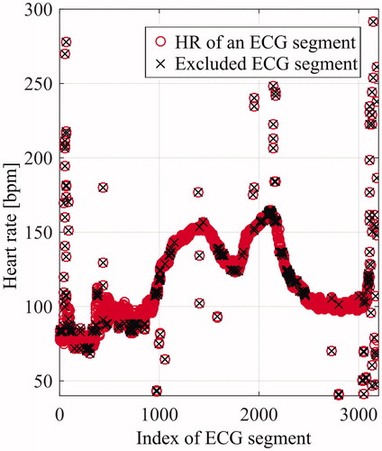
Figure 5. 3 D representation of all templates for one ECG recording overlaid with characteristic points from the IBT toolbox. As one can observe from the graph, the detectable points correlate with the minima and maxima (valleys and mountains). This depiction is referred to as 3 D ECG. (a) Top view for better legibility. HR: Heart rate.

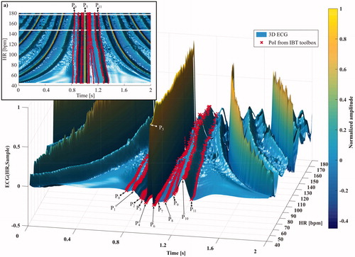
Figure 6. Depiction of timings for the waves and spikes within an ECG segment with respect to heart rate. Data from ECG recordings of the training set (group A) are depicted as points. Furthermore, polynomial fits of this work are compared with the square root and linear fits introduced by Burke & Nasor [4,7]. Thereby, deviations among the profiles are seen that are most obvious for the QRS-complex and the P- and T-waves, respectively. Bpm: Beats per minute.

Figure 7. Flowchart of the signal generation including optical readout and physical output. MATLAB software generates the synthetic ECG signal or outputs recorded data from a database. The selected signal is shown on-screen within the GUI and output through the sound card via the “sound” command. An external USB sound card converts the digital signal into an analogue signal before it reaches the external circuit board. Depending on the switch position, ECG or common-mode (CM) signals are available for system-testing. Calibration (Cal) uses switch position 1.

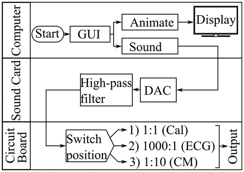
Figure 8. Circuit board to convert sound card signals to physiological ECG signals. (a) The circuit diagram of the board with three output options, adjustable with a switch (see Table 1 for details). (b) The manufactured circuit board with its outputs ‘1’ and ‘2’. Potentiometers allow for precise adjustment of attenuation/ amplification factors.

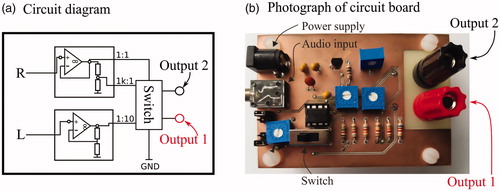
Table 1. Switch positions and associated modes of the circuit board.

Switch position	Output 1 (Electrode 1)	Output 2 (Electrode 2)	Comment
1	GND	50 Hz 1:1	Needed for calibrating the computer’s volume setting to 2 Vpp output
2	GND	ECG 1000:1	Configuration to scale ECG signals from 2 Vpp to 2 mVpp
3	CM 50 Hz	CM 50 Hz	Configuration to amplify CM signal from 2 Vpp to 20 Vpp

Mode 1 is required for calibration, mode 2 for ECG signal output and mode 3 for common-mode stability testing. Figure 8 introduces both the circuit diagram and realisation. CM: Common-mode.

Table 2. Correlation results for the training ECG recordings in group A.

ECGID: ECG recording within group A	ECG1 (rECG)	ECG2	ECG3	ECG4	ECG5	ECG6	ECG7	ECG8
Cross-Correlation: COR(rECG, ECGID) [%]	100.0	99.58	99.52	99.48	99.43	99.43	99.33	99.29

The correlation factors describe the similarity between each ECG recording with respect to the reference ECG (rECG).

Figure 9. Determination of the accuracy between recorded ECG signals with the profiles of this work and the profile suggested by Burke & Nasor [4,7]. To achieve an unbiased result, only the test set (group B) is evaluated for this comparison.

Table 3. Curve-fitting results for the third-order polynomials according at the function at bottom of the table (equivalent to Equation (3)(3) $$T_{\text{fit}}\left(\mathit{HR}\right)=a_3{\mathit{HR}}^3+a_2{\mathit{HR}}^2+a_1{\mathit{HR}}^1+a_0$$(3) ).

Heart-rate dependent profile for the	a3	a2	a1	a0
PQ-Interval TPQ-I(HR)	1.053e–07	−4.099e–05	0.004665	−0.009073
P-Wave TP(HR)	0	−2.755e–6	0.0005669	0.09601
PQ-Segment TPQ-S(HR)	9.777e–08	−3.556e–05	0.003804	−0.09485
QT-Interval TQT(HR)	0	0	−0.001248	0.4691
QRS-Complex TQRS(HR)	0	0	−3.07e–05	0.1104
ST-Segment TST(HR)	−2.334e–08	1.692e–05	−0.004021	0.3457
T-Wave TT(HR)	0	0	−0.000176	0.1581
Fitting curve for all individual segments: TFit(HR) = a3 HR³ + a2 HR² + a1 HR + a0

The temporal relation with respect to heart rate of each wave or spike is obtained individually by means of least squares approximation. Figure 1 introduces the basic morphology.

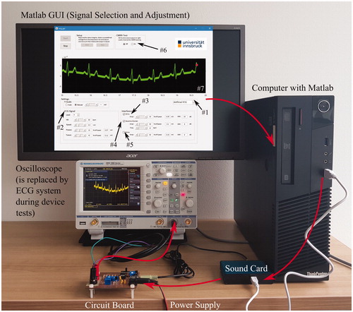
Figure 10. The entire ECG simulator system. Signals are selected (#1), or adjusted for synthetic ECG generation (#2–#6), via a MATLAB GUI. The computer running the software outputs these signals via the external sound card. Finally, the circuit board converts the signal intensities to physiological levels. The configuration above shows an oscilloscope (Rohde & Schwarz, HMO 1002) for demonstration purposes. For real ECG testing, the system under test is connected to the circuit board directly. The MATLAB display (#7) and the physical signal output are synchronised. The signal shown above is a synthetic ECG with 60 bpm, 50 Hz noise and baseline wander. An enlarged view of the GUI is included in the online supplement.

Burke MJ, Nasor M. An accurate programmable ECG simulator. J Med Eng Technol. 2001;25:97–102.

 PubMed Web of Science ®Google Scholar

Baas T. ECG based analysis of the ventricular repolarisation in the human heart. KIT Karlsruhe: University Press; 2012

 Google Scholar

Lenis G. Signal Processing Methods for the Analysis of the Electrocardiogram. Karlsruhe, Germany: Karlsruhe Institute of Technology; 2017

 Google Scholar

Burke MJ, Nasor M. Wavelet based analysis and characterization of the ECG signal. J Med Eng Technol. 2004;28:47–55.

 PubMedGoogle Scholar